
After the LEMONTREE annual meeting in Seoul, South Korea, which took place from 25 to 29 August 2025, I had the opportunity to stay in Seoul for another month and work in Youngryel’s group at Seoul National University.
During this time, I worked on developing an fPAR and LAI product that largely excludes anthropogenic influences on vegetation. The base data set for this project was the long-term fPAR and LAI product from 1982 to 2022 (Jeong et al., 2024).
We will use the final product from this secondment to benchmark and calibrate our P-model in the future. The advantage of this is that artificial irrigation, fertilisation, agricultural plant varieties and agrarian growth cycles are not included and therefore do not influence the signal. In Youngryel’s group, I had easy access to my basic data set, and Sungchan Jeong was always available to help me and answer my questions.
The Science Part
During the time in Seoul, we followed roughly six steps to create the ‘natural’ LAI and fPAR dataset.
- The project work began with a first step of getting familiarised with the LAI dataset. Its resolution is 0.05°, so we decided to process the land cover data at the same resolution. However, because a 0.25° resolution is easier to reuse and sufficiently fine for global simulations, we aggregated the 0.05° product to 0.25°.
- Secondly, we prepared the land cover data. First, we worked only with the ESA CCI LC data (Copernicus Climate Change Service, 2019) (CCI), and later with the GLC_FCS30D (Zhang et al., 2024) (GLC) and Land-Use Harmonisation (Hurtt et al., 2020) (LUH2). We aggregated the native 300m fine CCI data to 0.05° resolution annually. Then we extracted only the classes we were interested in: all agricultural pixels and all urban pixels. These are then aggregated across all years from 1992 to 2020 and compiled into a single static binary mask. Pixels are marked as ‘used’ if at least 10% of a 0.05° pixel has been marked as anthropologically influenced (either urban or agricultural) in at least three given years. We chose these thresholds to keep the mask as strict as possible: to remove as many anthropological pixels as possible without accidentally including outliers. In line with the CCI mask, we also created a GLC-based mask, which ultimately gave us another static mask.
- Then we created an ‘abiotic’ mask that excluded all CCI pixels that are predominantly ice, snow, wasteland or water. This mask was only created for a random year because it was only needed to remove regions such as oceans, permanent ice or deserts.
- We used the LUH2 dataset to mask regions that are pastures but are designated only as grassland in the GLC and CCI data. These regions mainly include pastureland. The LUH2 data contains fractional land cover information from 850–2100, annually, with a resolution of 0.25°. However, for our work, we only used data from 1992 to 2020. Initially, we aggregated all grassland pixels in the CCI dataset at resolutions of 0.05° to 0.25° for this time period. If the grass proportion for a given CCI pixel was at least 10% and the corresponding pixel in the LUH2 dataset was at least 10% pasture, we calculated the ratio of pasture to grass. If the ratio was at least 50%, the pixel was marked as ‘used’ and thus to be removed.

These four steps yielded four masks: two marking urban and agricultural areas (CCI and GLC-based), one marking unvegetated regions, and one marking pastureland.
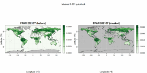
- The last two steps were applying the masks to the monthly LAI and fPAR data and aggregating the resulting product to 0.25° area-weighted. After further work back in Switzerland, this process resulted in eight outputs. LAI and fPAR at 0.05° and 0.25°, each masked once with the CCI mask and once with the GLC mask. In this final product, pixels that were classified mainly as agricultural, urban and pasture land are marked as N/A.
The Social Part!
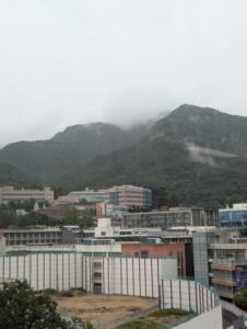
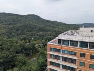
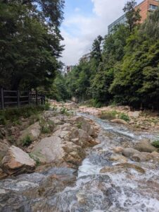
The SNU campus is located just outside the city, surrounded by green hills and hiking trails. On the western edge of the campus is Sillim Valley, through which a river flows, making it the perfect place to relax and cool off. Right next to this valley is the College of Agriculture and Life Sciences (CAS), where one of Youngryel’s group offices and my workplace were located on the 5th floor. From there, I had a great view of the surrounding landscape.
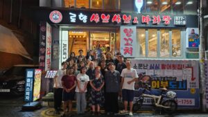
At first, I had to get used to the large office, where around 15 people worked together. It was quite a change from my office in Bern, which I usually share with only two other people. Nevertheless, the atmosphere was always calm and focused. I really enjoyed working in this research group, where everyone was always very friendly and helpful. Jisun, Sungchan and Gahyeon in particular helped me a lot, whether with advice on the project, ideas for excursions or recommendations for hairdressers and restaurants.
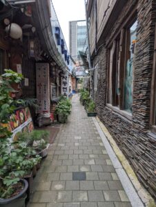
I was also able to talk regularly with Youngryel himself about my project and my stay, as well as my plans for my free time and the week’s holiday I had in Korea after the project. There is so much to see, experience and do in Seoul, which is why I made the hour-long journey from my Airbnb near the university into the city most weekends. Autumn had just begun, and after the summer heat, the temperatures had dropped to a pleasant level for me, inviting me to spend time outdoors. I often visited museums, wandered through the streets and alleys of Seoul, or tried out different restaurants.
Future Work & Thanks
Next, we will create further products, each with smaller and larger thresholds. We will then compare these with the original products. We will also compare the two mask types (based on CCI or GLC) to analyse where they differ. The final product will then be used as input to the P-model to calibrate it better.
I learned a lot about working with different raster data during this project. The process was sometimes relatively slow and required many revisions. For example, because something was not quite right somewhere in the code or because specific goals and steps were adjusted during the course of the project.
I want to express my sincere thanks to Youngryel and Youngryel’s group for their hospitality. I already miss my time in South Korea, and I will definitely return soon.
Ananda is a PhD student at the University of Bern, studying under the supervision of Prof. Dr. Benjamin Stocker. Ananda’s research focuses on vegetation modeling, particularly on developing a model-data integration framework for simulating global carbon, water, and nitrogen cycles.
Sources
- Copernicus Climate Change Service. (2019). Land cover classification gridded maps from 1992 to present derived from satellite observations Version 2.0.7cds. ECMWF. https://doi.org/10.24381/CDS.006F2C9A
- Copernicus Climate Change Service. (2019). Land cover classification gridded maps from 1992 to present derived from satellite observations Version 2.1.1. ECMWF. https://doi.org/10.24381/CDS.006F2C9A
- Zhang, X., Zhao, T., Xu, H., Liu, W., Wang, J., Chen, X., & Liu, L. (2024). GLC_FCS30D: The first global 30 m land-cover dynamics monitoring product with a fine classification system for the period from 1985 to 2022 generated using dense-time-series Landsat imagery and the continuous change-detection method. Earth System Science Data, 16(3), 1353–1381. https://doi.org/10.5194/essd-16-1353-2024
- Hurtt, G. C., Chini, L., Sahajpal, R., Frolking, S., Bodirsky, B. L., Calvin, K., Doelman, J. C., Fisk, J., Fujimori, S., Klein Goldewijk, K., Hasegawa, T., Havlik, P., Heinimann, A., Humpenöder, F., Jungclaus, J., Kaplan, J. O., Kennedy, J., Krisztin, T., Lawrence, D., … Zhang, X. (2020). Harmonisation of global land use change and management for the period 850–2100 (LUH2) for CMIP6. Geoscientific Model Development, 13(11), 5425–5464. https://doi.org/10.5194/gmd-13-5425-2020
- Jeong, S., Ryu, Y., Gentine, P., Lian, X., Fang, J., Li, X., … & Prentice, I. C. (2024). Persistent global greening over the last four decades using novel long-term vegetation index data with enhanced temporal consistency. Remote Sensing of Environment, 311, 114282. https://doi.org/10.1016/j.rse.2024.114282