The P model: challenges we face and plan to address

By Colin Prentice

Upscaling: From Leaf to Canopy

The P-model helps us to understand plant photosynthesis “writ large” (known as gross primary production, GPP) and so to bridge the gap from leaf-level processes to ecosystem-level measurements and global predictions. It starts with a pretty big assumption – the big leaf approximation. Essentially, we treat the entire canopy as if it’s just one giant leaf. There’s logic behind this – first articulated by (the late) Piers Sellers in the 1990s, although Graham Farquhar may have been the first to spell out the underlying mathematics.

Many empirical models use remotely sensed data on “greenness” to link GPP to absorbed light. Absorbed light is the product of incoming light and the fraction absorbed by green tissues, known as fAPAR, which is available from an increasing number of satellite-borne sensors. So-called light-use efficiency (LUE) models assume that GPP is equal to the product of absorbed light and LUE. This assumption has a strong empirical basis in findings on crop growth by John Monteith back in the 1970s. However, there are now many LUE models, which differ in how they estimate LUE.

At first sight, it seems counter-intuitive that GPP should be proportional to absorbed light. After all, it is well known that the response of photosynthesis to incident light is non-linear, saturating at high light. But that’s the instantaneous response, which doesn’t take account of the slower variation in photosynthetic capacity (known as photosynthetic acclimation) as light availability changes through the season; nor the analogous process by which leaves subject to different degrees of shading adopt photosynthetic capacities appropriate to their light environment. It turns out that for every light level, there is a photosynthetic capacity that yields a maximum rate of photosynthesis – once the finite cost of maintaining that capacity has been accounted for. And if leaves adopt that optimal capacity, the outcome – and this is a very robust mathematical result – is that leaf-level photosynthetic capacity is proportional to incident light. This is the original foundation of the P-model. The model typically runs on weekly to monthly timesteps because that is the time scale on which Rubisco activity adjusts to environmental variation. Moreover, this theoretical basis makes it possible to predict what LUE should be, directly from the standard (Farquhar-von Caemmerer-Berry, FvCB) model of photosynthesis. The close connection to the FvCB model distinguishes the P-model from all of the empirical LUE models.

Known and Unknowns in the FvCB Model

The FvCB model works well – although, like all models, it has limitations. The model includes some quantities that are reasonably well known and that do not vary massively among species, and others that do vary greatly and are unknown – unless you measure them directly, which is not an option for large-scale modelling.

Let’s start with the knowns.

Rubisco is the enzyme that fixes CO₂ for photosynthesis. Sometimes, Rubisco grabs an oxygen (O₂) molecule by mistake. This would not be important except for the fact that the amount of oxygen in the atmosphere is orders of magnitude greater than the amount of CO₂. Today’s atmosphere contains such a large amount of oxygen because of all the photosynthesis and carbon burial that has happened over billions of years. The oxygen concentration is large enough to result in a significant fraction of the gross CO₂ uptake being released, via the pathway called photorespiration.

The first known quantity is Γ*, the photorespiratory CO₂ compensation point – that is, the (leaf-internal) CO_2­ level at which photosynthesis is balanced by photorespiration. Γ* varies in predictable ways with temperature and oxygen partial pressure. It does vary among species, but for first-order global modelling, these variations can reasonably be ignored.

Next is K, the effective Michaelis-Menten coefficient of Rubisco. K, like Γ*, depends on both temperature and oxygen partial pressure. Its calculation depends on two quantities – the Michaelis-Menten coefficients for CO₂ and O_2­ respectively. Again, these quantities vary, but not hugely, among species.

Then there is φ₀, the maximum light-use efficiency of photosynthesis, only attained under low light and unstressed conditions. The theoretical absolute maximum value of φ₀ is 0.125, i.e. at least eight photons are needed to fix one carbon atom. In the original FvCB model this quantity is fixed, but under natural conditions, φ₀ also changes with temperature. We’ll return to this later.

Now the unknowns. These are trickier. They change based on temperature, but also vary widely between plants and as a function of growth conditions:

• V_cmax – the leaf-level maximum CO₂ fixation capacity, which depends on the activity of Rubisco.
• J_max – the leaf-level maximum electron transport capacity, which determines the photosynthetic rate under low light and depends on enzymes of the electron-transport chain, which convert light energy into chemical energy used for CO₂ fixation.
• χ – the ratio of leaf-internal to ambient CO₂ (always less than one during photosynthesis, because the stomata provide a resistance to the inward flow of CO₂). χ is determined by stomatal behaviour, which is tightly regulated by leaves.

These three quantities are crucial for making predictions with the FvCB model. But here’s the rub: nearly every complex ecosystem model uses FvCB (or some minor variation of it) but the models make different assumptions about these values. That’s probably the single most important reason why global models give inconsistent results.

Most land ecosystem models fix the values of V_cmax and J_max at 25°C (allowing actual values to vary with temperature, following their relatively well-known dependencies) for predefined plant functional types (PFTs). PFTs are the last refuge of the scoundrel, to borrow a phrase from Samuel Johnson, because they enable modellers to sidestep the lack of universal theory by empirically assigning different trait values to the plants that dominate in different regions of the world. Basically, PFTs group all plants into a few categories and assume their traits are constant. This works as a rough approximation, but it misses the continuous variation (in time as well as in space) that we see in nature. That’s where eco-evolutionary optimality (EEO) theory comes in. EEO just means that plants are not stupid! They acclimate and adapt to the environments where they live. This is a consequence of natural selection – the most fundamental law of biology.

What Makes the P-model Unique?

The P-model is built on three foundational hypotheses that explain how plants optimize their photosynthetic performance.

The Least-Cost Hypothesis posits that plants balance the capacity for water loss during transpiration (maintaining the pathway of water from roots to leaves) with the capacity for carbon fixation (maintaining active enzymes, including Rubisco), in such a way as to minimise the sum of the costs associated with both. This simple idea leads to a formula that correctly predicts how χ varies with the environment. When the air is dry, plants reduce χ, thereby conserving water. Under warm growth conditions, plants increase χ, because water transport becomes “cheaper” (thanks to the reduced viscosity of water) while photosynthesis becomes more expensive (thanks to increased photorespiration). At high altitudes, where photosynthesis is cheaper due to the low O₂ pressure, plants reduce χ – a fact known since the 1980s (from an elegant measurement campaign by Christian Körner) and now, finally, fully explained by the least-cost hypothesis.

The Coordination Hypothesis describes how plants fine-tune their photosynthetic machinery to match light availability. This hypothesis proposes that V_cmax takes the value that results in full use of available light. This adaptability ensures resource use is maximised without waste. It results in a simple proportionality between photosynthetic capacity (at the growth temperature) and the light intensity experienced by leaves.

The Cost-Benefit Hypothesis predicts the ratio between the maximum electron transport rate (J_max) and V_cmax, based on the idea that leaves should balance the cost of maintaining J_max (assumed to be proportional to J_max) and the benefit (taken to be the electron-transport limited rate of photosynthesis).

Together, these hypotheses provide a robust framework, allowing the P-Model to predict gross primary production (GPP) across diverse ecosystems with remarkable accuracy.

 

Strengths of the P-model

With its basis in optimality principles, the P-model moves away from PFTs and instead adopts universal, continuous, adaptive responses of plants to environmental conditions. This approach allows the model to be applied without change in different biomes. The model’s simplicity is a major practical advantage. Unlike models requiring long lists of parameters per PFT, the P-model requires only (a) information on fAPAR and (b) a small set of environmental variables (light, temperature, atmospheric pressure, vapour pressure deficit and soil moisture).

The model’s predictions have shown strong agreement with empirical observations, including spatial and temporal trends in stable carbon isotope discrimination (a proxy for χ) and photosynthetic capacity. And whereas most models are hampered by their use of fixed parameter values (such as V_cmax at 25˚C) for PFTs, the dynamic responses of GPP and leaf traits to a changing environment – including rising CO₂ – emerge organically from the structure of the P-model. Thus, the P-model is also expected to enhance the reliability of predictions of ecosystem responses to future scenarios.

Challenges and Limitations

Despite its strengths, there are known issues with the P-model as currently formulated.

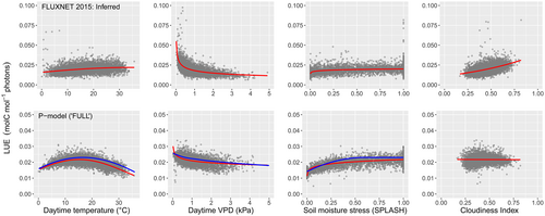
One area of concern is the model’s temperature-dependent predictions of GPP, which indicate a fairly steep decline in LUE at temperatures above about 20˚C. This conflicts with observations of relatively stable GPP in warm environments (see Fig. 1 below). We are exploring adjustments to address this issue. Our first line of attack is on the temperature dependence of φ₀, which currently follows experimental determinations on tobacco plants carried out by Carl Bernacchi in the early 2000s. We are working on a much more comprehensive, ecosystem-level determination of the temperature response of φ₀, based on an analysis of net ecosystem exchange measurements at eddy-covariance flux tower sites across the world.

 

Another limitation, also evident in Fig. 1, is the model’s inability to account for the diffuse radiation effect, whereby LUE increases under cloudy conditions due to the more effective penetration of diffuse light into dense canopies. A two-leaf model, differentiating between sunlit and shaded leaves, provides a potential solution that has been shown to work well in other contexts and is being implemented now in the P-model.

The representation of water stress also poses challenges. The current approach yields inconsistent results in arid environments, highlighting the need for refined soil moisture corrections that separate impacts on φ₀ and the parameters of the least-cost model.

Further discrepancies arise in specific biomes. The model overestimates spring GPP in colder regions, likely due to simplified assumptions about how photosynthetic capacity changes during early leaf development. Addressing this issue will require improved modelling of the seasonal dynamics of leaf absorptance and chlorophyll content. Conversely, in the wet tropics, GPP estimates tend to fall short. This may partly be due to biases in satellite-derived inputs during the wet (cloudy) season, when valid data are sparse. Integrating other sources of remote sensing data, and attention to improving gap-filling algorithms, may help resolve this issue.

Finally, the model’s current global GPP predictions (~100 PgC/year) fall below widely accepted values (120–150 PgC/year). Revisiting optimality criteria and testing model sensitivity to CO₂ levels could uncover underlying causes and pave the way for more accurate estimates.

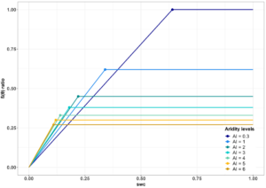
A sub-daily version of the P-model has been developed to capture instantaneous responses to environmental changes, allowing predictions of daily GPP cycles. The refinement of water stress functions, such as Giulia Mengoli’s breakpoint model (see Figure 2 below), introduces a systematic variation of LUE response curves with climatological aridity. Accounting for the bell-shaped temperature response based on eddy-covariance flux data, and shifting focus to leaf temperature rather than ambient temperature, will help to enhance the model’s alignment with real-world processes.

 

The Path Ahead

The P-model’s ongoing evolution reflects a broader effort to merge theoretical rigour with empirical realism. By addressing the model’s current limitations—from temperature responses to water stress and light dynamics—it is poised to become an even more powerful tool for understanding plant behaviour in a changing world. It’s all about finding the right balance between trade-offs. Plants have been doing that quite successfully for millions of years. We need to catch up!