By Nancy Nichols
Should you care about the numerical accuracy of your computer? After all, most machines now retain about 16 digits of accuracy, but usually only about 3 – 4 figures of accuracy are needed for most applications; so what’s the worry? To demonstrate, there have been a number of spectacular disasters due to numerical rounding error. One of the most well known is the failure of a Patriot Missile to track and intercept an Iraqi Scud missile in Dharan, Saudi Arabia, on February 25, 1991, resulting in the deaths of 28 American soldiers.

The failure was ultimately attributable to poor handling of rounding errors. The computer doing the tracking calculations had an internal clock whose values were truncated when converted to floating-point arithmetic with an error of about 2-20 . The clock had run up a time of 100 hours, so the calculated elapsed time was too long by 2-20 x 100 hours = 0.3433 seconds, during which time a Scud would be expected to travel more than half a kilometer.
(See The Patriot Missile Failure)
The same problem arises in other algorithms that accumulate and magnify small round-off errors due to the finite (inexact) representation of numbers in the computer. Algorithms of this kind are referred to as ‘unstable’ methods. Many numerical schemes for solving differential equations have been shown to magnify small numerical errors. It is known, for example, that L.F. Richardson’s original attempts at numerical weather forecasting were essentially scuppered due the unstable methods that were used to compute the atmospheric flow. Much time and effort have now been invested in developing and carefully coding methods for solving algebraic and differential equations such as to guarantee stability. Excellent software is publicly available. Academics and operational weather forecasting centres in the UK have been at the forefront of this research.
Even with stable algorithms, however, it may not be possible to compute an accurate solution to a given problem. The reason is that the solution may be sensitive to small errors – that is, a small error in the data describing the problem causes large changes in the solution. Such problems are called ‘ill-conditioned’. Even entering the data of a problem into a computer – for example, the initial conditions for a differential equation or the matrix elements of an eigenvalue problem – must introduce small numerical errors in the data. If the problem is ill-conditioned, these then lead to large changes in the computed solution, which no method can prevent.
So how do you know if your problem is sensitive to small perturbations in the data? Careful analysis can reveal the issue, but for some classes of problems there are measures of the sensitivity, or the ‘conditioning’, of the problem that can be used. For example, it can be shown that small perturbations in a matrix can lead to large relative changes in the inverse of the matrix if the ‘condition number’ of the matrix is large. The condition number is measured as the product of the norm of the matrix and the norm of its inverse. Similarly small changes in the elements of a matrix will cause its eigenvalues to have large errors if the ‘condition number’ of the matrix of eigenvectors is large. Of course to determine the condition numbers is a problem implicitly, but accurate computational methods for estimating the condition numbers are available .
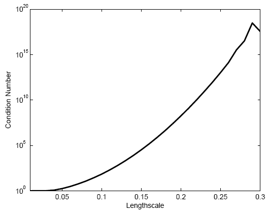
An example of an ill-conditioned matrix is the covariance matrix associated with a Gaussian distribution. The following figure shows the condition number of a covariance matrix obtained by taking samples from a Gaussian correlation function at 500 points, using a step size of 0.1, for varying length-scales [1]. The condition number increases rapidly to 107 for length-scales of only size L = 0.2 and, for length scales larger than 0.28, the condition number is larger than the computer precision and cannot even be calculated accurately.
This result is surprising and very significant for numerical weather prediction (NWP) as the inverse of covariance matrices are used to weight the uncertainty in the model forecast and in the observations used in the analysis phase of weather prediction. The analysis is achieved by the process of data assimilation, which combines a forecast from a computational model of the atmosphere with physical observations obtained from in situ and remote sensing instruments. If the weighting matrices are ill-conditioned, then the assimilation problem becomes ill-conditioned also, making it difficult to get an accurate analysis and subsequently a good forecast [2]. Furthermore, the worse the conditioning of the assimilation problem becomes, the more time it takes to do the analysis. This is important as the forecast needs to be done in ‘real’ time, so the analysis needs to be done as quickly as possible.
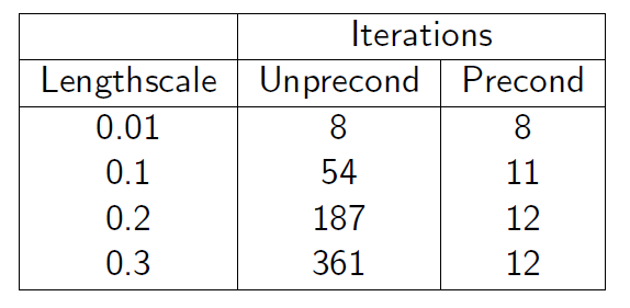
One way to deal with an ill-conditioned system is to rearrange the problem to so as to reduce the conditioning whilst retaining the same solution. A technique for achieving this is to ‘precondition’ the problem using a transformation of the variables. This is used regularly in NWP operational centres with the aim of ensuring that the uncertainties in the transformed variables all have a variance of one [1][2]. In this table we can see the effects of the length-scale of the error correlations in a data assimilation system  on the number of iterations it takes to solve the problem, with and without preconditioning of the problem [1]. The conditioning of the problem is improved and the work needed to solve the problem is significantly reduced. So checking and controlling the conditioning of a computational problem is always important!
[1] S.A Haben. 2011. Conditioning and Preconditioning of the Minimisation Problem in
Variational Data Assimilation, University of Reading, Department of Mathematics and Statistics, Haben PhD Thesis
[2] S.A. Haben, A.S. Lawless and N.K. Nichols. 2011. Conditioning of incremental variational data assimilation, with application to the Met Office system, Tellus, 63A, 782–792. (doi:10.1111/j.1600-0870.2011.00527.x)
