by Chris Thomas
An interesting problem in climate science is working out what happened in the world’s oceans in the last century. How did the temperature change, where were the currents strongest, and how much ice was there at the poles? These questions are interesting for many reasons, including the fact that most global warming is thought to be occurring in the oceans and learning more about when and where this happened will be very useful for both scientists and policymakers.
There are several ways to approach the problem. The first, and maybe the most obvious, is to use the observations that were recorded at the time. For example, there are measurements of the sea surface temperature spanning the entire last century. These measurements were made by (e.g.) instruments carried on ships, buoys drifting in the ocean, and (in recent decades) satellites. This approach is the most direct use of the data, and arguably the purest way to determine what really happened. However, particularly in the ocean, the observations can be thinly scattered, and producing a complete global map of temperature requires making various assumptions which may or may not be valid.
The second approach is to use a computer model. State-of-the-art models contain a huge amount of physics and are typically run on supercomputers due to their size and complexity. Models of the ocean and atmosphere can be guided using our knowledge of factors such as the amount of CO2 in the atmosphere and the intensity of solar radiation received by the Earth. Although contemporary climate models have made many successful predictions and are used extensively to study climate phenomena, the precise evolution of an individual model run will not necessarily reproduce reality particularly closely due to the random variation which often occurs.
The final technique is to try to combine the first two approaches in what is known as a reanalysis. The process of reanalysis involves taking observations and combining them with climate models in order to work out what the climate was doing in the past. Large-scale reanalyses usually cover multiple decades of observations. The aim is to build up a consistent picture of the evolution of the climate using observations to modify the evolution of the model in the most optimal way. Reanalyses can yield valuable information about the performance of models (enabling them to be tuned), explore aspects of the climate system which are difficult to observe, explain various observed phenomena, and aid predictions of the future evolution of the climate system. That’s not to say that reanalyses don’t have problems, of course; a common criticism is that various physical parameters are not necessarily conserved (which can happen if the model and observations are radically different). Even so, many meteorological centres around the world have conducted extensive reanalyses of climate data. Examples of recent reanalyses include GloSea5 (Jackson et al. 2016), CERA-20C, MERRA-2 (Gelaro et al. (2017)) and JRA-55 (Kobayashi et al. (2015)).
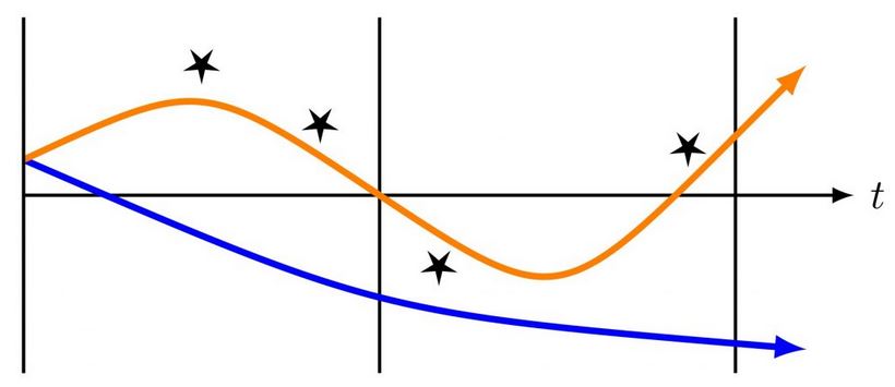
When performing a reanalysis the observations are typically divided into consecutive “windows” spanning a few days. The model starts at the beginning of the first window and runs forward in time. The reanalysis procedure pushes the model trajectory towards any observations that are in each window; the amount by which the model is moved depends on how much we believe the model is correct instead of the observation. A very simplified schematic of the procedure can be found in Figure 1.

This takes us to the title of the post. Obviously it’s not actually possible to use data from the future (without a convenient time machine), but the nice aspect of a reanalysis is that all of the data are available for the entire run. Towards the start of the run we have knowledge of the observations in the “future”; if we believe these observations will enable us to push the current model closer to reality it is desirable for us to use them as effectively as possible. One way to do that would be to extend the length of the windows, but that eventually becomes computationally unfeasible (even with the incredible supercomputing power available these days).
The question, therefore, is whether we can use data from the “future” to influence the model at the current time, without having to extend the window to unrealistic lengths. The methodology to do this has been introduced in our paper (Thomas and Haines (2017)). The essential idea is to use a two-stage procedure. The first run is a standard reanalysis which incorporates all data except the observations that appear in the future. The second stage then uses the future data to modify the trajectory again. Two stages are required because the key quantity of interest is the offset between the future observations and the first trajectory; without this, we’d just be guessing how the model would behave and would not be able to exploit the observations as effectively.
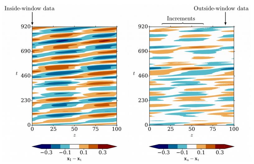
Our paper describes a test of the method using a simple system: a sine-wave shape travelling around a ring. Observations are generated at different locations and the model trajectory is modified accordingly. It is found that including the future observations improves the description relative to the first stage; some results are shown in Figure 2. The method has been tested in a variety of situations (including different models) and is reasonably robust even when the model v aries considerably through time.

We have now implemented the method in a large-scale ocean reanalysis which is currently running on a supercomputer. We are particularly interested in a process known as the AMOC (Atlantic Meridional Overturning Circulation) which is a North-South movement of water in the Atlantic Ocean (see Figure 3 for a cartoon). It is believed that the behaviour of water in the northernmost reaches of the Atlantic can influence the strength of circulation in the tropical latitudes; crucially, this relationship is strongest at a time lag of several years (Polo et al. (2014)). Data collected by the RAPID measurement array in the North Atlantic (www.rapid.ac.uk) take the role of the “future” data in the reanalysis and are used to modify the model trajectory in the North Atlantic. The incorporation of RAPID data in this way has not been done before and we’re looking forward to the results!

References
Jackson, L. C., Peterson, K. A., Roberts, C. D. and Wood, R. A. 2016. Recent slowing of Atlantic overturning circulation as a recovery from earlier strengthening. Nat. Geosci. 9(7), 518–522. http://dx.doi.org/10.1038/ngeo2715
Kobayashi, S. et al. 2015. The JRA-55 Reanalysis: General specifications and basic characteristics. J. Meteor. Soc. Japan Ser. II 93(1), 5–48. http://dx.doi.org/10.2151/jmsj.2015-001
Gelaro, R. et al. 2017. The Modern-Era Retrospective Analysis for Research and Applications, Version 2 (MERRA-2) J. Clim. 30(14), 5419–5454. http://dx.doi.org/10.1175/JCLI-D-16-0758.1
Thomas, C. M. and Haines, K. 2017. Using lagged covariances in data assimilation. Accepted for publication in Tellus A.
Polo, I., Robson, J., Sutton, R. and Balmaseda, M. A. 2014. The Importance of Wind and Buoyancy Forcing for the Boundary Density Variations and the Geostrophic Component of the AMOC at 26°N. J. Phys. Oceanogr. 44(9), 2387–2408. http://dx.doi.org/10.1175/JPO-D-13-0264.1
