The first paper of my PhD, “A data-model approach to interpreting speleothem oxygen isotope records from monsoon regions on orbital timescales”, is available online at Climate of the Past Discussions (https://doi.org/10.5194/cp-2020-78). In this paper, I utilised >150 speleothem oxygen isotope (δ18O) records from the SISAL (Speleothem Isotope Synthesis and Analysis) database to constrain the large-scale (global and regional) trends in monsoon climate in the past, focusing on orbital-scale changes, namely evolution through the Holocene epoch and signals through the mid-Holocene, Last Glacial Maximum and Last Interglacial. These observations were compared to water isotope enabled climate models to investigate the climatic drivers of these trends.
This data-model approach is exciting because it allows us to disentangle the many processes that can influence speleothem δ18O variability, spanning climate processes such as precipitation and circulation changes, to karst and cave processes. By combining numerous speleothem records to construct large-scale trends, we can minimise the site-specific influence of karst and cave processes that can often complicate the interpretation of individual speleothem δ18O records. Meanwhile, exploration of isotope-enabled palaeoclimate simulations allows us to investigate the contribution/role of individual climate drivers to these large-scale trends.
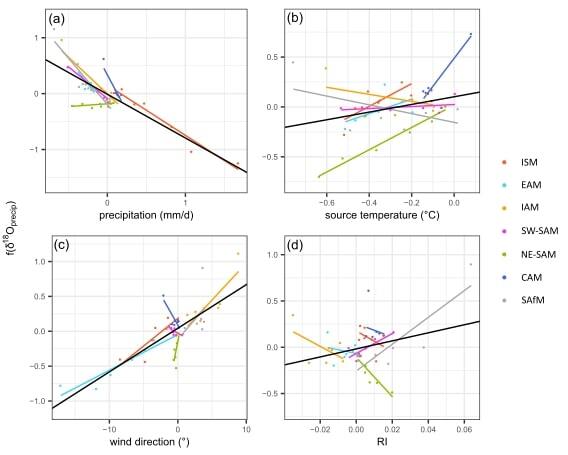
Figure 1 below shows composite speleothem δ18O trends for several regional monsoons, compared to simulated δ18O of precipitation trends through the Holocene epoch. In figure 2, we have separated out the key drivers of these simulated δ18O trends using multiple linear regression, illustrating the importance of precipitation amount and circulation changes (and to a lesser degree, temperature changes) to monsoon δ18O (orbital-scale) variability.
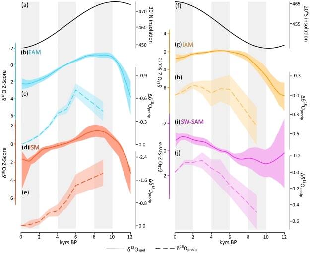
Figure 1: Evolution of regional speleothem δ18O signals through the Holocene compared to δ18Oprecip simulated by the GISS model. The left panel shows northern hemisphere monsoons (EAM = East Asian Monsoon; ISM = Indian Summer Monsoon) and summer (May through September) insolation at 30° N (Berger, 1978). The right panel shows southern hemisphere monsoons (SW-SAM = southwest South American Monsoon; IAM = Indonesian-Australian Monsoon) and summer (November through March) insolation for 20° S (Berger, 1978). The speleothem δ18O changes are expressed as z-scores, with a smoothed loess fit (3,000 year window), and confidence intervals obtained by bootstrapping by site. δ18Oprecip values are expressed as anomalies from the pre-industrial control simulation. Note that the isotope axes are reversed, so that the most negative anomalies are at the top of the plot, to be consistent with the assumed relationship with the changes in insolation.