Finally… long in the making, my “method” paper is out in Quaternary Research http://dx.doi.org/10.1017/qua.2020.44 today. It could not have been completed without a great deal of help from my co-authors and colleagues. My thanks to them all.
I work on what the pollen from long cores from lake-beds can tell us about the climate of Southern Europe during the last glacial period, and the forerunner of this paper was a poster at last year’s EGU in Vienna. The pollen data come from cores among the 93 in the ACER (Abrupt Climate Changes and Environmental Responses) database (Sanchez Goñi et al. 2017a, b).
Many palaeoclimate reconstructions are qualitative, where the pollen spectra are interpreted by, for instance, associating more trees with warmer wetter climate. Quantitative reconstructions, giving numbers for the climate, are relatively rare (and I’m beginning to understand why), but are valuable input to model-data comparisons; the last glacial is particularly useful because it experienced climates well outside the limits of those in the instrumental record, and also rapid changes (Dansgaard-Oeschger cycles) similar in speed and amplitude to those expected under current warming.
My reconstructions of climate use what seems initially to be a straightforward transfer function, applying the relationship between modern climate and different types of modern pollen to the pollen in the cores. This works because plants tend to be most abundant around their favourite parts of whatever climate gradients they care about (unimodal distribution).
The method I use is Weighted Averaging Partial Least Squares (WA-PLS), developed by among others Cajo ter Braak, who, pleasingly, was one of the reviewers of the paper; Colin Prentice was involved in its genesis, and it is still being improved – Mengmeng Liu is working with Colin and Cajo on a variant. WA-PLS is not the only reconstruction game in town, but many points in the paper apply to any method that uses modern pollen, or indeed other biological material such as diatoms.
“Seems” straightforward: not quite so fast. There are quite a few choices to make if you want a robust answer, and often reconstruction papers say little to nothing about how these choices were made, or their potential consequences. First is the climate that your modern pollen set covers: if you use, say, samples collected only around the Mediterranean, then you can’t be sure that you will see the full realised niches of the plants – where is the cold climate, if you want to reconstruct the last glacial? You want samples covering the whole range of climate that could be important, and you could plot the climate space to show this. In Figure 1, EMB is a Mediterranean set and doesn’t cover cold climates: no good for glacial work, but SMPDS is promising.
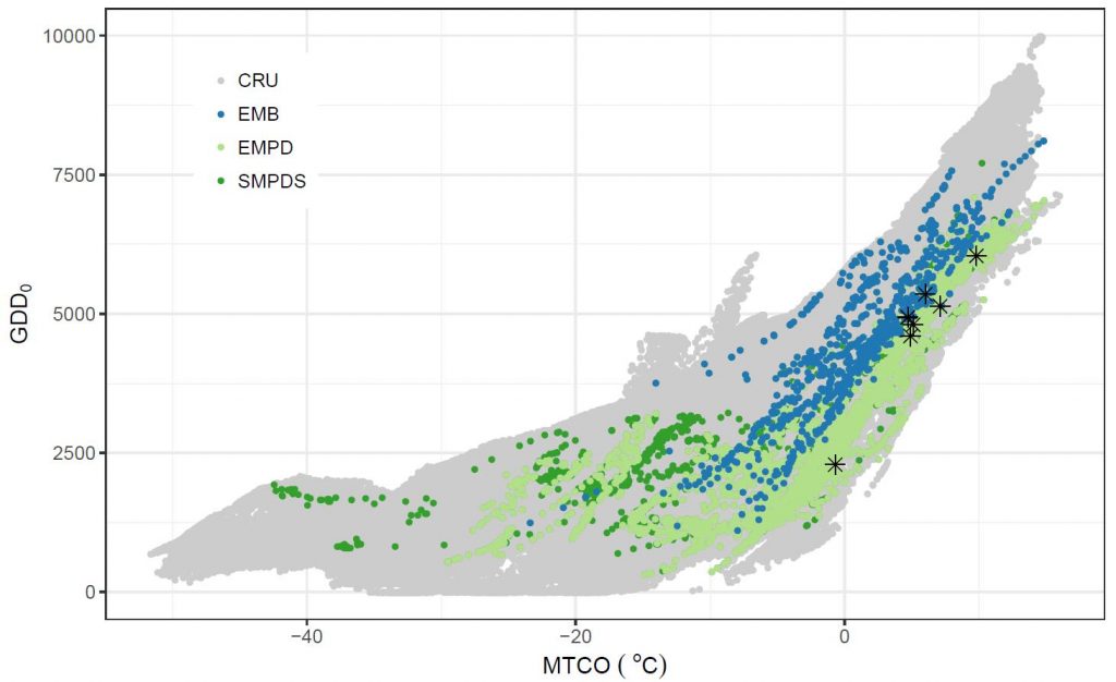
Figure 1. Distribution of modern pollen samples in climate space, represented by growing degree days above 0 oC (GDD0) and mean temperature of the coldest month (MTCO), sampled by EMBSECBIO (EMB), the European Modern Pollen Database (EMPD), and the full SMPDS (SMPDS) data sets. Stars indicate the present climate at the fossil sites used as examples.
So the length of climate gradient you sample is important. Secondly, it is not the sheer number of samples that matters, but the continuity along the gradient: unsampled gaps in the gradient confuse WA-PLS, which expects an approximately unimodal distribution.
Another key issue is how many, and which, pollen taxa you use. The fewer the number of samples for a given taxon, the less reliable the climate information it gives. One way round this is to rely on “niche conservatism”, the habit of closely related plants to like the same climate. So by combining related taxa, having checked that they do in fact have similar preferences, you can get a more precise estimate of climate. Although there is a tendency to ignore taxa which are either unhelpfully prolific like Pinus, or seem uninformative because they are widely tolerant or scarce, we found that generally it was better to leave them in: more is better.
Bootstrapping the modern pollen set gave us a view of the reliability of the climate estimates for each taxon, and hence of the reliability of the climate reconstructions sample-by-sample down the core. This means that if the reconstruction spread gets suspiciously wide at some point, you can track down the culprit taxa and work out if there may be a good physical reason to ignore them. In Fig 2, the SMPDS set with its wider climate range and better sampling of taxa gives a much narrower spread than the less comprehensively sampled EMB and EMPDS sets. And the weird increase in uncertainty in b around 70 ka can be pinned down to one very rare taxon.
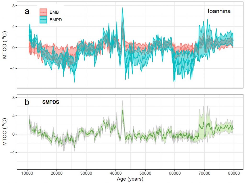
Figure 2. Reconstructions of mean temperature of the coldest month (MTCO) during the last glacial period (80,000 to 10,000 calendar years before 2000) using the pollen record from Lake Ioannina, (a) using the EMBSECBIO (EMB) and the European Modern Pollen Database (EMPD) as training data sets, and (b) using the full SMPDS data set. The reconstruction spread (±2σ) is obtained by resampling the training set 1,000 times.
Perhaps the oddest result was that the standard WA-PLS model statistical diagnostics are not a good guide to the suitability of the choices, which is a snare for the innocent user. This is because the model can only say how well it replicates the modern pollen set it was given: give it a pollen set from a climate which is obviously too restricted for your p urposes, and it may tell you it is excellent.
I’m now working on improving age-depth models, so that reconstructions can be directly compared across a region. An early version of this was a “display” at this year’s online EGU, which can be accessed here: https://meetingorganizer.copernicus.org/EGU2020/EGU2020-2691.html