
by Javier Amezcua, February 2025
My name is Javier Amezcua and I am currently an Associate Professor at Universidad Iberoamericana in Mexico City. I spent 10 years at the University of Reading as part of the Data Assimilation Centre. Here I describe some of the work I started there, in collaboration with the University of Oslo and the Norwegian Seismic Array. This is an ongoing collaboration.
The challenge of predicting …
Forecasting the future state of the atmosphere is a challenge. In mathematical terms, it is an initial value problem that requires a set of initial conditions and a mathematical model that correctly represents the time evolution of the atmospheric physical variables. Let us focus on the former: how are these initial conditions found?
… starts with observing
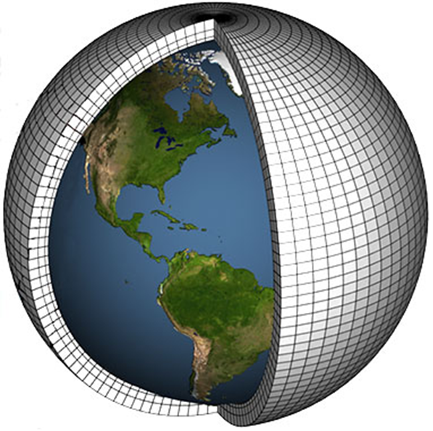
The atmosphere is a continuum represented mathematically (and then computationally) as a set of boxes in a 3D grid. The finer the grid, the more processes we can resolve and the closer we get to reality. To predict the evolution of the atmosphere, we must populate every single box with the values of the corresponding physical variables: horizontal wind (2 components), vertical wind, temperature, pressure, density and water content. This is a monumental task, since we cannot directly observe these variables everywhere, we must fill many of these values from models or climatology. However, the correct use of real observations is paramount since they give information about what the atmosphere is really doing. This is particularly crucial in chaotic systems where states diverge from each other.
Observing the atmosphere
Weather stations allow for direct observations of the variables in some locations at the Earth’s surface. Direct observations at other heights can be obtained launching radiosondes in meteorological balloons, a colossal world-wide coordinated effort performed every 6 hours by national meteorological centres. These balloons usually reach heights of up to ~20 km before exploding and plunging back to the surface. Airplanes also take measurements in their flight paths. All of these observations are extremely useful but limited.
There are remote ways to measure the atmosphere, including Doppler radars and satellite observations. The latter have been an invaluable source of information about the atmosphere in the last 40 years. These are indirect observations that contain integrated information of an atmospheric slab. We have learned how to extract useful information from them in successful non-trivial ways [1].
All of the previous observations, however, are concentrated in the troposphere (the lowest atmospheric layer, roughly below 12 km). Even the satellite observations have more ‘sensitivity’ in tropospheric levels. The stratosphere (the next layer, roughly up to 50 km) is very poorly observed. This is a shame since knowing its state can help us predict e.g. cold spells over Europe two weeks in advance [2]. In August 2022, the European Space Agency (ESA) launched the AEOLUS mission. This carried a wind lidar (laser radar) capable of measuring winds up to roughly a height of 40km, covering the lower stratosphere. This mission ended in April 2023, and unfortunately a replacement will not be coming until the end of this decade. We have a huge observational gap in the stratosphere — can we do something with observational datasets we already have?
The music of the atmosphere: infrasound
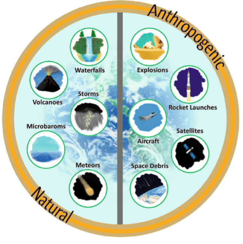
Infrasound waves are mechanical waves with low frequencies (0.1-1 Hz). They are inaudible to human beings but audible to some animals like bees and hippopotamuses. Their dissipation is low (dissipation is a power of frequency), so they can travel hundreds or thousands of kilometers and still be coherently detected by arrays. Infrasound waves can be produced naturally (earthquakes, volcanic eruptions, ocean microbaroms) or by human sources (aircrafts, rocket launches, explosions).
There is an amazing set of acoustic arrays around the world which can detect infrasound. Part of this is the result of the United Nations CTBT (Comprehensive Nuclear-Test-Ban Treaty), which prohibits nuclear tests. These arrays are constantly checking the compliance to this treaty, but as a byproduct they deliver continuous acoustic monitoring of the atmosphere.
Explosions that become tomographies
Infrasound waves interact with the atmosphere as they travel through it, if a wave encounters a headwind, its effective velocity will diminish. If, on the contrary, it encounters a favourable tailwind, it will travel faster. If it encounters a cross wind, its apparent direction of arrival will be shifted. This can all be detected with the acoustic arrays mentioned above, and we can make use of infrasound measurements as if these waves were taking a tomography of the atmosphere. In fact, this is not too different from the integrated quantities involved with satellites, and we can use the expertise developed in that field to help with infrasound observations.
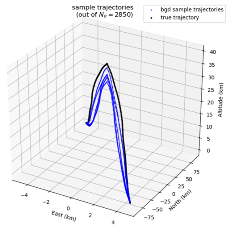
A difficulty in the process just mentioned is that we have to know the exact location and emission time of the infrasound wave. Another stroke of luck has provided us with this perfect study case. Different countries have accumulated ammunition which expires after a certain date. For safety reasons, they have to detonate these ammunitions on a regular basis. We have been working with two datasets: one of Finnish explosions with detections in Norway, roughly 179 km North of the explosion site, and the other of explosions in Oklahoma with detections roughly 256 km West of the explosion site. Figure 3 shows some simulations of the infrasound propagation for the Finnish case.
Our work is in a preliminary state, but we have shown that it is possible to update three variables in an atmospheric column (temperature and the two horizontal winds) knowing three observations (travel time, change in back azimuth angle and apparent velocity of the received waves) [3,4,5]. Our plan is to continue this research until this type of observation can be used in NWP. We have recently started collaboration with the Woods Hole Oceanographic Institute in Massachusetts and the Centre for Nuclear Energy in Paris.
[1] Campbell, W. F., C. H. Bishop, and D. Hodyss, 2010: Vertical covariance localization for satellite radiances in ensemble Kalman filters. Mon. Wea. Rev., 138, 282–290, https://doi.org/10.1175/2009MWR3017.1.
[2] Baldwin, M. P., D. B. Stephenson, D. W. J. Thompson, T. J. Dunkerton, A. J. Charlton, and A. O’Neill, 2003: Stratospheric memory and skill of extended-range weather forecasts. Science, 301, 636–640, https://doi.org/10.1126/science.1087143.
[1] Amezcua J, Näsholm S, Blixt EM, Charlton-Perez AJ. Assimilation of atmospheric infrasound data to constrain tropospheric and stratospheric winds. QJR Meteorol Soc. 2020; 146: 2634–2653. https://doi.org/10.1002/qj.3809
[2] Amezcua, J. & Barton, Z.(2021) Assimilating atmospheric infrasound data to constrain atmospheric winds in a two-dimensional grid. Q J R Meteorol Soc, 147(740, 3530–3554. Available from: https://doi.org/10.1002/qj.4141
[3]Amezcua, J., S. P. Näsholm, and I. Vera Rodriguez, 2024: Using Satellite Data Assimilation Techniques to Combine Infrasound Observations and a Full Ray-Tracing Model to Constrain Stratospheric Variables. Mon. Wea. Rev., 152, 1883–1902, https://doi.org/10.1175/MWR-D-23-0186.1.


