
by Giovanni De Cillis(1) and Alberto Carrassi(1,2),March 2025
(1): Dept of physics, U Bologna, IT (2): Visiting Professor at U of Reading, UK
Our research aims to develop a hybrid, physics and data-driven, model for the sea ice, as part of the project MELTED, in collaboration with CMCC and Politecnico di Milano.
Why hybrid modeling?
Like for other components of the earth system, physics-based sea ice numerical predictions are affected by errors of different nature including discretization errors, imperfect parametrizations or inaccurate boundary conditions and forcings. Sea ice modeling presents additional complexities due to its multiscale, multiphase, discontinuous nature.
Data assimilation (DA) comes in handy, by leveraging observational data to constrain and improve numerical predictions [1]. Moreover, the remarkable advancements of machine learning (ML) along with the growing availability of satellite observations, enabled the development of hybrid models — physics-based numerical models augmented through ML. This is often represented by some parametrization being replaced by an ML model [2]. An alternative class of hybrid models relies on the combination of DA and ML, where the ML component is designed to account for all the errors affecting the physical core [3] [4]. Our work falls into this latter category.
Column physics test bench
The methodology is developed in the idealized scenario of the 1D sea ice vertical column physics Icepack model [5]. The ice column model comprises five ice thickness categories, each discretized into seven ice layers and one snow layer. Heat and mass fluxes at the top surface boundary are derived from ERA5 reanalyses, while at the bottom boundary, the model is coupled to a slab ocean model with constant salinity. Observations are produced synthetically by running Icepack with a given parameters’ setup, while the forecast model differs from the “true” by some perturbed parameter. We focus on perturbing snow conductivity and maximum melting snow grain size, known to be among the most important parameters [6]. The ML model we wish to develop is meant to act as an additive correction to the forecast obtained by the incorrect model.
Figure 1 shows how the training data are produced and how a perfect hybrid model should work. The assumption of perfect initial conditions allows us to bypass DA and rule out the effect of initial condition error.
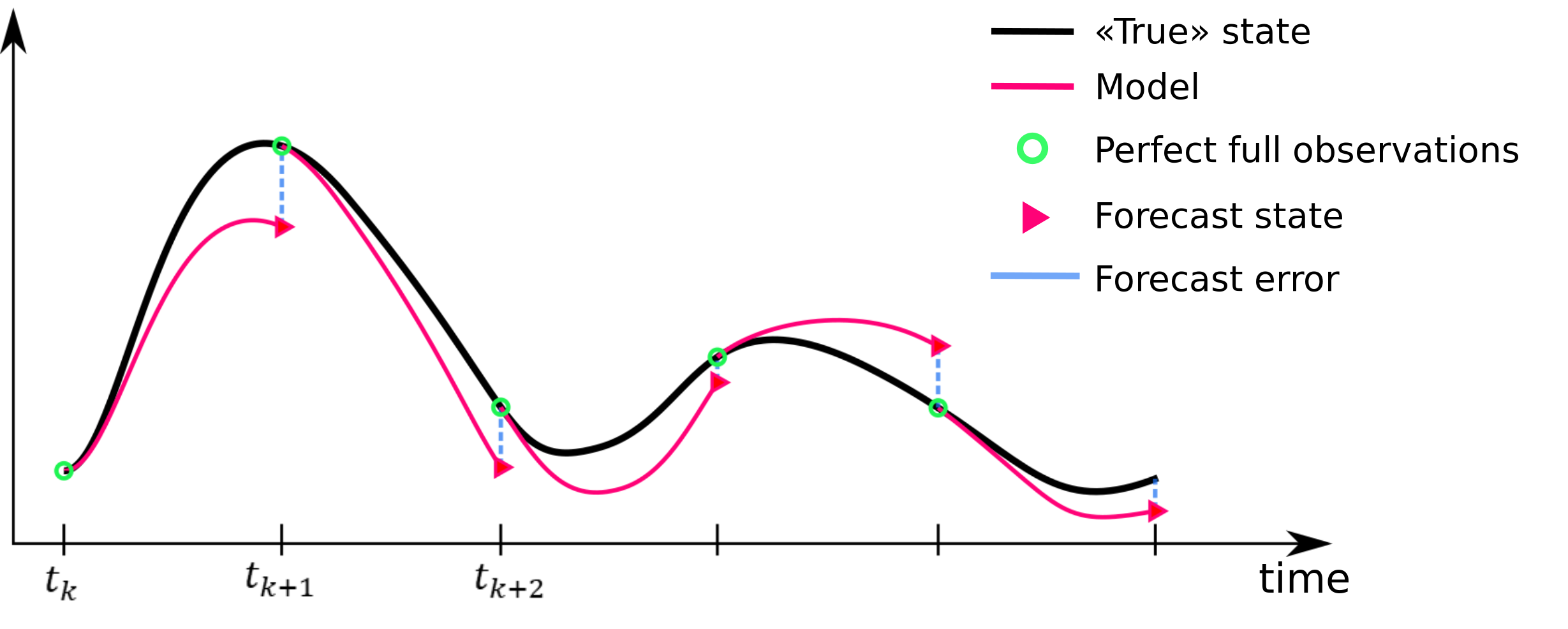
The training dataset is then constructed by collecting forecast states, forcings, and forecast errors at 60-days lead time across multiple locations over a 10-year period.
Hybrid Icepack model
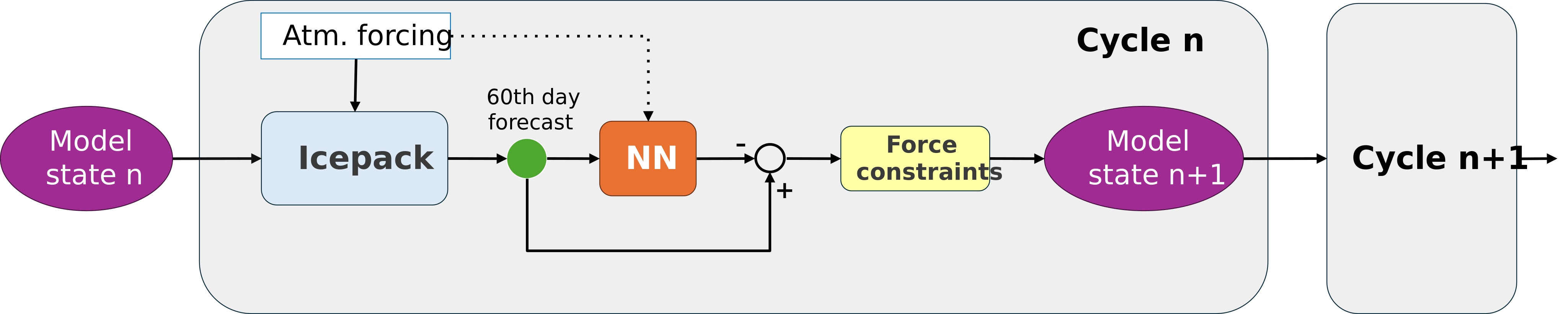
The hybrid model we developed corrects at each iteration only ice concentration and ice volume for all ice thickness categories, while keeping the remaining model state variables unchanged. We trained two separate neural networks (NN) to independently correct ice concentration and ice volume. These NN take as inputs the forecast state and the atmospheric forcing and output the forecast errors.
The hybrid model (Figure 2) concatenates the NN corrections to the forecast state. The NN are trained without any physical constraint, therefore there is no guarantee that the resulting corrected states are physically consistent. A post-processing step is required, where certain constraints are imposed, such as the ice concentration and volume being non-negative.
Online execution of the hybrid model
After training and validation, the hybrid model is tested over a period of 4 years against the uncorrected model and the true state. The results in Figure 3 show that the hybrid model substantially reduces the forecast error at time horizons much longer than the 60-days lead time. The hybrid model is stable even though only two variables of the model state are updated by the NN. Results suggest that the methodology is robust with respect to initial condition errors, that were absent in the training but occur after the first hybrid iteration. Despite the idealized scenario, this study provides valuable insights into the significance of features for correcting specific model errors and the sensitivity to forcing and initial condition errors.

References
[1] A. Carrassi, M. Bocquet, L. Bertino and G. Evensen, “Data assimilation in the geosciences: An overview of methods, issues, and perspectives,” WIREs Climate Change, vol. 9, p. e535, 2018.
[2] S. Driscoll, A. Carrassi, J. Brajard, L. Bertino, M. Bocquet and E. Ö. Ólason, “Parameter sensitivity analysis of a sea ice melt pond parametrisation and its emulation using neural networks,” J. Comput. Sci., vol. 79, p. 102231, 2024.
[3] J. Brajard, A. Carrassi, M. Bocquet and L. Bertino, “Combining data assimilation and machine learning to infer unresolved scale parametrization,” Philosophical Transactions of the Royal Society A: Mathematical, Physical and Engineering Sciences, vol. 379, p. 20200086, 2021.
[4] T. S. Finn, C. Durand, A. Farchi, M. Bocquet, Y. Chen, A. Carrassi and V. Dansereau, “Deep learning subgrid-scale parametrisations for short-term forecasting of sea-ice dynamics with a Maxwell elasto-brittle rheology,” The Cryosphere, vol. 17, p. 2965–2991, 2023.
[5] E. Hunke, R. Allard, D. A. Bailey, P. Blain, A. Craig, F. Dupont, A. DuVivier, R. Grumbine, D. Hebert, M. Holland, N. Jeffery, J.-F. Lemieux, R. Osinski, T. Rasmussen, M. Ribergaard, L. Roach, A. Roberts, A. Steketee, M. Turner and M. Winton, CICE-Consortium/Icepack: Icepack 1.4.1, Zenodo, 2024.
[6] J. R. Urrego-Blanco, N. M. Urban, E. C. Hunke, A. K. Turner and N. Jeffery, “Uncertainty quantification and global sensitivity analysis of the Los Alamos sea ice model,” Journal of Geophysical Research: Oceans, vol. 121, p. 2709–2732, 2016.


