by Jochen Broecker, March 2024
The Industrial Revolution saw not only the introduction of steam engines but also the introduction of anthropogenic air pollution due to the burning of fossil fuels, some of it coming from the running of steam engines. Clearly, problems with air pollution have been around since humans learned to control fire. However, the industrial revolution really took this to another level with the extraction and burning of fossil fuels (mainly coal). I do not know what fraction of coal production went into running steam engines compared to other industrial or domestic uses of coal (such as producing steel or heating cities), but if you ever took a ride on a museum steam train you will know that even the local pollution it creates merely through soot particles is very considerable already.
There is another link however between steam engines and air pollution that goes via data assimilation, as has turned out recently in our research. At first, steam engines were employed to pump excess water from mine shafts. But by converting the reciprocating motion of the piston into rotational power, the field of application greatly widened to grinding, weaving, and milling. A single large steam engine could drive entire factories via systems of transmission belts and shafts.
The need for speed (regulation)
Yet this brought about a problem: with individual machines on the factory floor being switched on and off, the demand for power varies in time, and with it the rotational speed of the steam engine. This creates problems in the production process. The steam engine needs to be regulated to provide a constant rotational speed at the output shaft independent of the load.
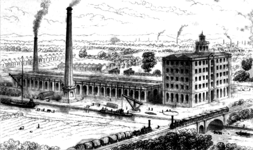
 Boulton & Watt engine of 1788
For this purpose, James Watt devised a contraption called centrifugal governor, which has as its most important component a pair of “fly balls” fixed to levers on a vertical shaft which in turn is connected to the output shaft of the steam engine. This device, first described by Christiaan Huygens but probably invented by Dutch millwrights, effectively measures the rotational speed of the output shaft. (Watt in fact never claimed credit for this component, but rather for its use in regulating steam engines.) A system of levers allows for the opening or closing of the steam valve using the measured speed. Thus the steam is fed to the engine in proportion to the error between the desired and the actual speed.
The beginnings of modern control theory
Although this contraption greatly improved the situation, it does not in fact reduce the error to zero. The mathematical analysis of this and other governors was carried out in a landmark paper by J.C. Maxwell [1] which is typically regarded as laying the foundations of modern control theory. In modern language, Maxwell uses linear stability theory to analyse proportional and proportional-integral control. In proportional (or P) control, the feedback signal is proportional to the error between the desired and the actual state, as in the governor described above. However, in proportional-integral (or PI) control, the feedback is proportional to a linear combination of the error and its integral over time. As Maxwell emphasises, a governor using PI control can restore the desired speed without error.
The reason behind this is that regulating a steam engine is a control problem with an unknown parameter, namely the load. The PI controller is, in a sense, equivalent to a simple P controller but with the unknown parameter regarded as an additional state of the dynamics. When configured correctly, the controller will provide an estimate of the load and, using that estimate, control the speed at the output shaft more accurately than a simple P controller.
From controlling steam engines to understanding air pollution
Data assimilation has control theory as one of its ancestors. In some of our recent research, however, the connection with PI controllers and, curiously, with atmospheric pollution, is more direct. So-called transport equations model the dispersal of atmospheric pollutants (such as soot, greenhouse gases, and harmful chemicals). The equations use reconstructed atmospheric wind fields to advect (i.e. carry along with it) the relevant substance. More complex models involve several pollutants possibly reacting with one another, or they consider how the pollution feeds back onto the atmospheric dynamics.
Our recent research considers such equations, and the challenge to reconstruct the distribution of the pollutant from sparse measurements. In addition, we want to reconstruct the source of the pollutant, which appears as a (multi-dimensional) parameter in the transport equations. We are currently investigating several approaches which, as it turns out, have a lot in common with the good old PI controller. Again, we consider the unknown parameters as additional dynamical degrees of freedom. Then we apply a very simple data assimilation approach using linear (or proportional) error feedback. The parameter estimates we obtain in this way are proportional to the error integrated over time.
In the context of our somewhat idealised equations, we can reconstruct the sources of the pollutant without any error. Since atmospheric transport models are partial differential equations, we need to use modern methods in partial differential equations in our analysis. Yet eventually we apply arguments from dynamical stability theory, which Maxwell’s paper was so instrumental in motivating.
[1] Maxwell James Clerk 1868. On governors. Proc. R. Soc. Lond.16270–283. http://doi.org/10.1098/rspl.1867.0055