by Tristan Quaife, March 2024
In Data Assimilation it is often necessary to assimilate observation types that are related to, but not directly predicted by, the underlying process model. Achieving this requires the use of observation operators, which transform the model state vector to predict an observed quantity. Simple examples might include averaging in space or interpolating in time to provide a better match with satellite data. However, observation operators can also be employed for much more complex tasks. This blog post explores some of the issues around using non-linear observation operators for assimilating certain types of satellite data into land surface models.
Researchers have devoted substantial effort to deriving products from satellite data that describe physical properties of the land surface. A common example is leaf area index, or LAI, which is also a key variable in land surface models. Since the launch of the MODIS sensors, over 20 years ago, there has been a large increase in such data being made readily available and hence they are an attractive source of observations for Data Assimilation. However, satellites themselves don’t actually measure these variables; they measure the amount of energy incident on the sensor, often reported as a radiance. To derive variables like LAI, some form of transformation is required, which typically involves a model that relates the observed radiances to the physical property of the surface. And, as with all models, they contain assumptions.
If products derived in this way are assimilated into a land surface model, there is no guarantee that the assumptions in the land model itself are consistent with the assumptions in the satellite data retrieval. In the worst-case scenario, this can lead to biases in the analysis. Taking MODIS LAI as an example, it contains explicit assumptions about the physical properties of the surface, such as the spatial distribution of the vegetation and its optical properties. Land models necessarily contain assumptions about these things too. In the case of LAI this can lead to biases in the amount of absorbed sunlight calculated by the model, which has onward impacts on other processes such as the surface temperature and the rate of photosynthesis.
An alternative approach is to forward model quantities which are closer to the raw observations of the satellite, using an observation operator. Ideally, this would be the at-sensor radiances, but that can add a lot of additional complexity. A reasonable middle ground is to use surface-leaving radiances or reflectance. The operators for this problem are examples of radiative transfer models. Their use does not negate the need to remove conflicting biases, but provides a physically based solution to this problem. A key concept, therefore, is that radiative transfer models used in this context should be derived from the same set of assumptions as within the model. In that way, it is possible to ascribe any systematic discrepancies between the model and the observations after Data Assimilation to the model itself.
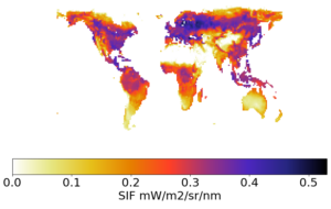
This all sounds very complex, but the good news is that most land surface models already contain radiative transfer models. They must do, to solve the surface energy balance. For many types of satellite data, this means assimilating them can be done with only minor modifications to the existing model code. For example, solar induced fluorescence, or SIF, is gaining lots of attention currently and is commonly used as a proxy for photosynthesis, which itself is an important variable in many land models and often used in data assimilation for carbon cycle problems. But, as we don’t have reliable models to predict photosynthesis from SIF, it is better to predict the SIF from the land surface model and assimilate the SIF observations. As most land models already have routines to calculate the transport of electromagnetic radiation in plant canopies, it is reasonably straightforward to adapt them for this purpose. Figure 1. shows an example of SIF predicted from the UK land surfaces model, JULES, using an observation operator that is physically consistent with the land model itself.