by Ross Bannister, April 2025
The method of least squares (or MLS, Barlow, 1993) is at the very centre of variational data assimilation (or “Var”, Schlatter, 2000). Var is one of the major data assimilation (DA) approaches used in numerical weather prediction (NWP) to estimate a model’s state from observations. The basic idea of Var is to find a model’s state – let’s call this x – that agrees as closely as possible with observations – let’s call these y. The invention of the MLS is credited to mathematicians Legendre and Gauss near the turn of the 19th century.
The basic principle of least squares
The MLS relies on predicting what the observations ‘ought’ to be given the model’s state. In DA terminology this uses the ‘observation operator’, often written mathematically as H(x). The predicted observations will be different from the actual (measured) observations. The MLS poses the question: what x minimises the objective function ½|y – H(x)|2, where | |2 takes the sum of the squares of the differences between elements of y and H(x).
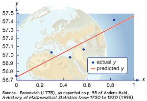
Imagine we have a simple model with one grid box and two variables: T0 (starting temperature) and dtT (how fast the temperature changes over time). We also have observations of temperature at the grid box at times in the future, namely y1 = Tob1 at t = t1, y2 = Tob2 at t = t2, etc. We ask the question: what values of T0 and dtT best match the observations? The prediction of the first measured temperature is H1(T0, dtT) = dtT×t1 + T0, and similarly for the remaining observations. Readers who are familiar with the equation of a straight line “y=mx+c” may see parallel with our observation operator. It is therefore instructive to represent the observation operator as a straight line with gradient dtT and intercept T0. See the Fig 1. for the graphical interpretation, where the best fit dtT and T0 are found.
Figure: Movie illustration of the method of least squares to find the two parameters dtT and T0 from observations of T.
Beyond the straight line
The straight line is often a student’s first taste of the MLS, but least squares is more than that.
Firstly, x can contain more than two variables. In NWP x comprises billions of variables, essentially representing the values of multiple physical quantities in each model grid box.
Secondly, the operator H(x) is not limited to linear relationships. There are many instances in NWP where observation predictions are non-linearly related to model variables. Perhaps the simplest is for an observation of the wind speed. Wind speed is related to the east-west (u) and north-south (v) wind components via √(u2 + v2). Other examples of non-linear components of H(x) are more complex. For example, the prediction of quantities that a satellite would see (radiances, Eyre, 1989), and the NWP model itself when observations are at a later time than the model state to be determined (Pires et al., 1996). Whatever the form of H(x), one can attempt to minimise the objective function using a descent algorithm. However, this is harder when H(x) is non-linear as non-linearity can lead to multiple minima (Pires et al., 1996).
Thirdly, in general not all observations should play an equal role in estimating x. In a diverse observing system observations will come from instruments with a range of precisions. The MLS can account for instrument precision by weighting the contributions to the objective function according to the inverse square of each observation’s error. This results in low precision observations (high error) having less influence than high precision observations. This is weighted least squares, which can be generalised to ideas around error covariances of the observations and naturally links to ideas of likelihood (maximum likelihood estimates).
Fourthly, the standard MLS accounts for uncertainty in the observations, but not in the time that they are made (ti). Accounting for uncertainty in the times adds another layer of complexity to the problem, e.g. Orear, 1982.
Equifinality and null spaces
Equifinality is the idea that many situations can lead to the same result. In MLS, this happens when more than one x leads to the same minimum value of the objective function. When H(x) is linear, this is connected to the concept of a null space. Think of x as existing in a multi-dimensional space. The null space consists of the directions in that space that lead to the same value of the objective function. In NWP, Var problems have a null space as there are far more variables in x than observations in y. To solve this we add an extra term to the objective function. The new term penalises deviations from a known first-guess state (the background state, xb). The objective function becomes ½|y – H(x)|2 + ½|x – xb|2 weighting the observations and the background state.
Conclusions
Using and understanding the MLS can be complex, and whole books cover the subject, e.g. Lewis et al., 2006. Nevertheless, it remains a powerful and effective tool in DA.
References
Barlow RJ, Statistics: a guide to the use of statistical methods in the physical sciences, volume 29, John Wiley & Sons, 1993.
Eyre JR, Inversion of cloudy satellite sounding radiances by nonlinear optimal estimation. I: Theory and simulation for TOVS. Quarterly Journal of the Royal Meteorological Society, 115, 1001-1026, 1989.
Lewis JM, Lakshmivarahan S, and Dhall S, Dynamic data assimilation: a least squares approach, volume 13. Cambridge University Press, 2006.
Orear J, Least squares when both variables have uncertainties. American Journal of Physics, 50, 912-916, 1982.
Pires C, Vautard R, and Talagrand O, On extending the limits of variational assimilation in nonlinear chaotic systems. Tellus A, 48, 96-121, 1996.
Schlatter TW, Variational assimilation of meteorological observations in the lower atmosphere: a tutorial on how it works. Journal of atmospheric and solar-terrestrial physics, 62, 1057-1070, 2000.


