
by Peter Jan van Leeuwen(1), April 2025
(1): Department of Atmospheric Science, Colorado State University, Colorado, USA
In a blog post dated 16 April 2025, Amos Lawless provided a valuable introduction to the challenge of using data assimilation to improve predictions of the coupled atmosphere-ocean system. In this post, I will highlight some recent developments addressing this issue.
Why is the coupled atmosphere-ocean system difficult?
The atmosphere and ocean differ significantly in both spatial and temporal scales. The atmosphere is mainly driven by large-scale high- and low-pressure systems spanning over 1,000 km and lasting a few days. In contrast, ocean eddies are smaller—around 50–100 km—and can persist for several weeks. As a result, ocean motions tend to be slower and more localized than those in the atmosphere.
Most data assimilation methods rely on covariances to spread observation information throughout the system. Covariances describe how two variables co-vary: if one changes, the other typically changes in response. These co-variations are dictated by the underlying physics. For instance, pressure gradients are closely tied to wind velocities due to the geostrophic balance—a principle that applies in both atmospheric and oceanic contexts.
If an observation alters the pressure at a particular location, covariances determine how other variables are physically linked to that change, and how much they should adjust. This allows us to update variables that aren’t directly observed by using the relationships encoded in the model’s covariances. To manage noise in these estimated covariances, many systems apply localization—artificially tapering covariances beyond a certain distance to prevent spurious, physically implausible updates.
This brings us to the core challenge of atmosphere-ocean data assimilation: the ocean and atmosphere exhibit different length scales, meaning their covariances also differ in scale. So, when an observation (e.g., sea-surface temperature) influences both systems, it raises a critical question—should we use atmospheric or oceanic covariances to distribute the information? Or should we apply an average that reflects both?
A potential solution to the covariance length-scale problem
One promising approach is to sidestep the length-scale issue entirely. As noted earlier, assimilation systems only need to know which variables strongly co-vary with observations—not their physical separation. Thus, a straightforward solution is to update only those variables that exhibit strong covariances with the observed ones.
In practice, rather than covariances, we use correlations—which are scaled covariances. These correlations vary over time and are difficult to prescribe in advance. However, modern assimilation techniques typically use an ensemble of model simulations. This allows for real-time estimation of correlations at each observation time step directly from the ensemble.
There’s more: some assimilation methods use observations collected over a time window to update the system state at a specific moment. This often yields more accurate results. However, estimating how observations at one time relate to model variables at another is complex. These relationships are influenced by atmospheric and oceanic flow, which evolve dynamically and unpredictably. Our new method addresses this by using the actual values of the correlations over space and time. If the correlation between an observation and a variable at a different time is small, no update is made. If it’s large, the system applies an appropriate update—naturally adapting to flow-dependent dynamics.
A simple example
Figure 1 presents simulations of a simplified model representing the atmosphere (left) and ocean (right). The horizontal axis indicates space, and the vertical axis represents time. Note how atmospheric features are larger and evolve faster compared to the ocean.
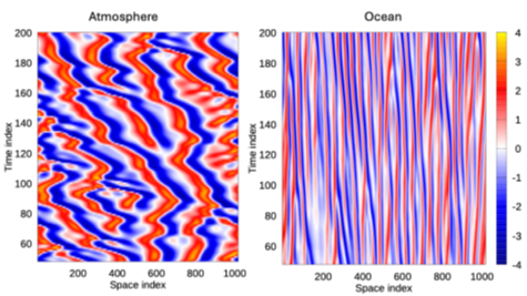
Figure 2 shows the correlations between a central observation (black circle) and all other atmospheric and oceanic variables. This illustrates that correlations depend on the evolving state of the system and highlights the importance of including temporal correlations—often overlooked in traditional approaches.
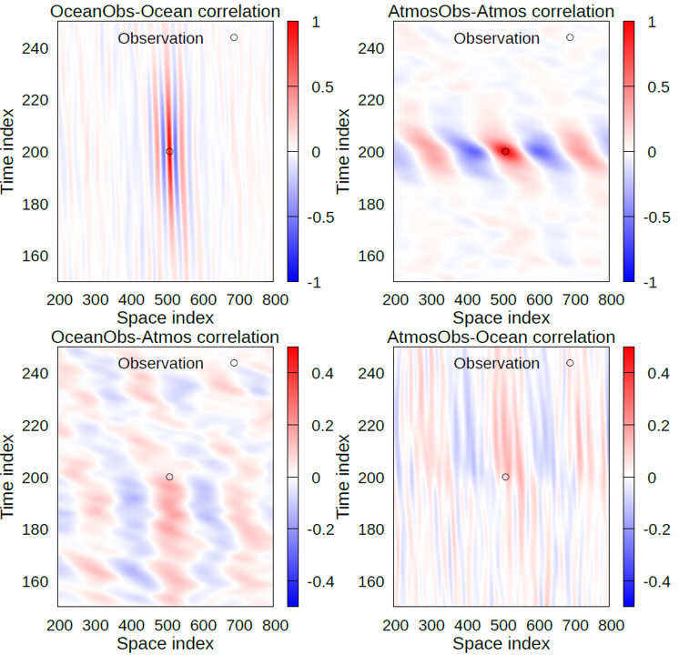
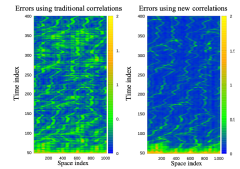
Figure 3 compares prediction errors in the atmospheric component using traditional length-scale-based correlations versus our new correlation-value-based method. The results clearly show significantly reduced errors with the new approach.
Looking ahead
This simple example demonstrates that using correlation values—rather than fixed length scales—can improve forecast accuracy and address key shortcomings in traditional methods. While the new approach is computationally more intensive, we are exploring optimizations to ensure it remains efficient. If successful, this method could substantially advance coupled atmosphere-ocean forecasting.
This blog is based on: Vossepoel, F.M, G. Evensen, and P.J. van Leeuwen (2025) Adaptive correlation- and distance-based localization for iterative ensemble smoothers in a coupled nonlinear multiscale model, which will soon appear in Monthly Weather Rev.