by Ross Bannister, April 2026
The circulation of the atmosphere plays an important role in the global distribution of trace gases, including carbon dioxide, methane, and other, perhaps less well-known, gases such as carbonyl sulfide. These gases exist naturally through biological processes, but also have artificial sources. Because of this, they can help us understand the Earth’s carbon cycle and identify artificial emissions. Winds transport these gases from their release (mainly at the Earth’s surface) to other locations where they can be measured, commonly by satellite.
Inverse modelling
The following question is often asked. How well can the locations and `strengths’ of the source (and sink) of a trace gas be determined using just measurements of the gas and knowledge of its predicted routes through the atmosphere? In other words, how reliably can we link emissions to the observed spatial distributions of the gas?
Scientists have studied this problem for some decades. They use methods known as `flux inversions’ or `inverse modelling’. This terminology owes its name to a kind of inverse (or reverse) of the usual way that modelling is done. The `usual’ way often termed forward modelling. Forward models try to predict the distribution of trace gases. They do this given (i) its initial conditions, (ii) its boundary conditions (namely the surface fluxes), and (iii) rules that govern the transport and chemical processes in the atmosphere. The `inverse’ of this process attempts to estimate (i) and (ii). It does this using knowledge of the distribution of the gas in the atmosphere in the form of observations. The forward model itself remains a component of the inverse model formulation. It needs to be an accurate reflection of reality for inverse models to be meaningful.
The flux inversion solution provides an estimate of the surface fluxes that are most consistent with the observations. The method accounts as much as possible for uncertainties (e.g. noise in the observations).
The EnviFlux tool
EnviFlux is a simplified flux inversion tool developed in NCEO. It is not intended to use real-world observations, but it is a valuable tool to help people understand the limitations of flux inversion and to test new ideas before running very expensive real-world systems.
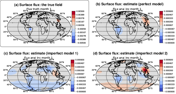
Consider the flux pattern in panel (a) of Fig. 1, comprising a source of a hypothetical trace gas in Eastern China and a sink over the Amazon. We use this as a hypothetical `true’ flux field and use it in a 100-day run of a 3D forward model (for simplicity this is a pure advection model using prescribed winds; also provided are some initial conditions). This allows the surface flux to influence the spatio-temporal distribution of the trace gas. Multiple observations of the resulting trace gas distribution are simulated. These are the simulated total column amount of the gas at locations under the path of a hypothetical polar orbiting satellite, making one observation every 96 seconds. Noise is added to the simulated observations to account for instrument noise.
We then do an experiment to ask the question: can EnviFlux recover the locations and strengths of the source/sinks by assimilating the noisy observations? This is done here with no prior knowledge of the true flux patterns in panel (a) (using a field of zero values for the prior flux field).
Panel (b) is EnviFlux’s result (EnviFlux incorporates the same forward model used to generate the observations, the `perfect model’ scenario). The locations of the fluxes are correctly identified, but their peak strengths are too low, and the length-scales are too large (but these mutually compensate to give correct total sources and sinks). This best-case result confirms that information about the about the (otherwise unknown) fluxes can, in principle, be inferred.
The impact of model error
In the real-world, however, we rarely have a forward model that is sufficiently good to deem it `near perfect’. In real-world models there are multiple issues such as incorrectly specified transport processes, e.g. imprecise resolved wind fields and unresolved winds associated with convection and turbulence.
Panels (c) and (d) are EnviFlux results using the same observations as in (b), but using incorrect winds in the forward model. True vertical winds are multiplied by 0.9 in (c) and 1.1 in (d). The incorrect transport causes the flux inversion to misinterpret the observations. As a result, source/sink patterns appear in the wrong locations, especially in (c).
Looking ahead
This illustrates a major concern. Clearly, transport errors need to be accounted for to avoid such misinterpretations. Currently, there are few ideas to account for these beyond reducing the influence of observations that are in danger of being misinterpreted. The solution will require either more sophisticated methods, and more accurate forward models. The latter could, in principle, be done with machine learning methods that are trained on the real (observed) evolving fields of trace gases in the atmosphere.
Clearly, there is a need to do further research to enable reliable and robust surface flux estimates to be made.
Reference
The EnviFlux tool is currently under peer review:
egusphere.copernicus.org/preprints/2026/egusphere-2025-6352/