By Yumeng Chen, January 2026.
Limitations of the normal distribution in data assimilation
Operational data assimilation methods typically perform best when both background (forecast) and observation errors can be approximated by a normal distribution. The normal distribution has many attractive mathematical properties. For example:
- It is fully characterised by its mean and (co)-variance.
- Its mean, mode, and median all coincide.
However, a limitation of the normal distribution is that it allows both positive and negative values. This assumption is inappropriate for many strictly non-negative weather and climate variables. For example, we do not expect negative rainfall or cloud cover.
How could we handle log-normal variables?
To address this issue, a common approach is to transform the original variable into a new variable that follows a normal distribution. Data assimilation is then performed for the transformed variables, and the resulting analysis is converted back to the original variable. This approach is known as Gaussian anamorphosis.
Operational marine ecosystem forecasting systems routinely assimilate phytoplankton. These are often considered to be log-normally distributed. This can be transformed to a normal distribution.
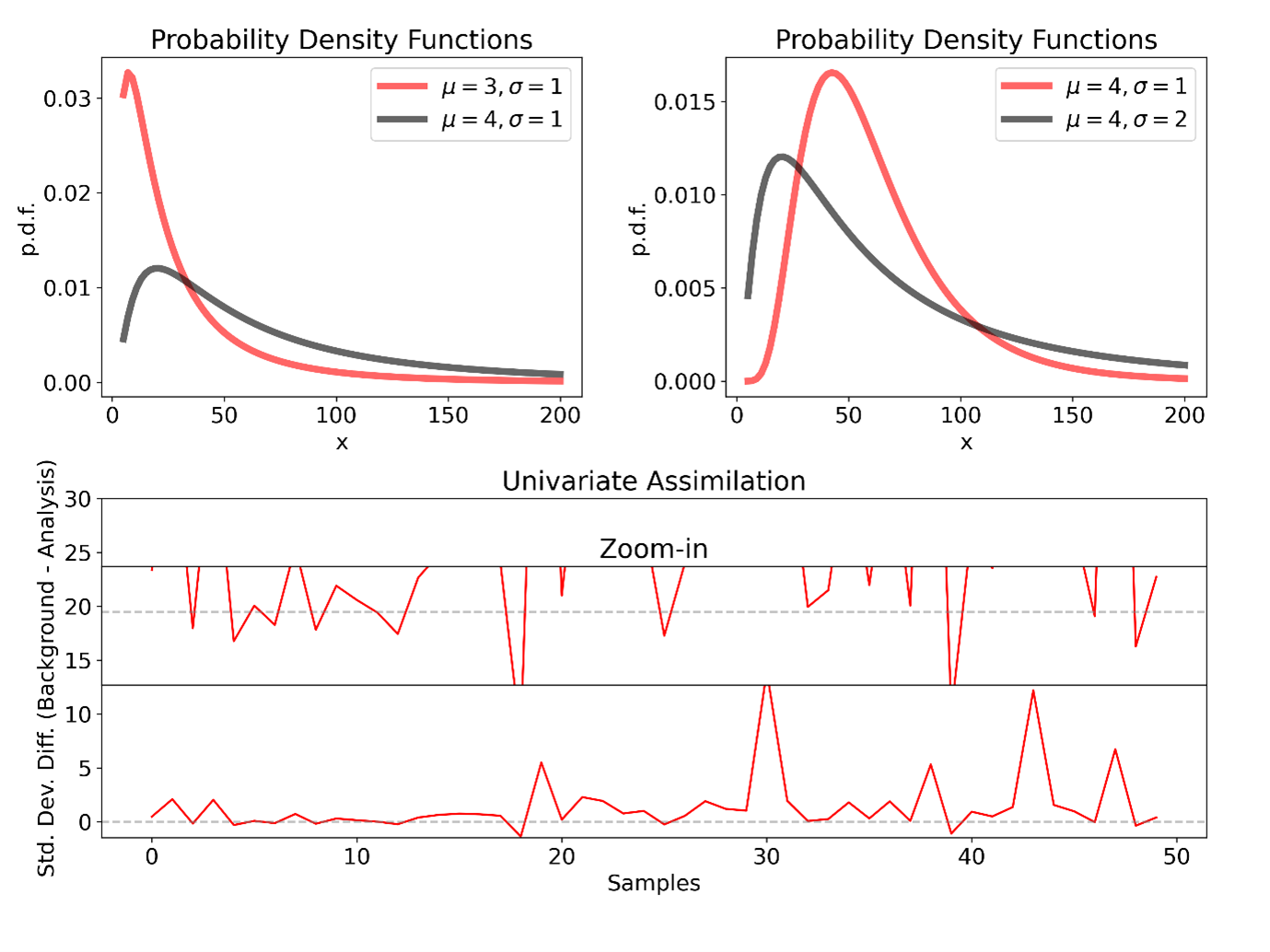
In the one-dimensional case, the mean (μ) and variance (σ2) of the associated normal distribution fully determine the log-normal distribution. For a normal distribution, μ defines the location of the distribution, while σ controls the spread.
The shape of a log-normal distribution behaves differently. While μ still controls the median of the distribution, both μ and σ influence its variance, mean, and mode. With fixed σ, increasing μ not only shifts the distribution but also broadens it. Likewise, with fixed μ, σ controls the variance of the log-normal distribution (see Figure 1).
Are analyses always less uncertain than the background?
What does this imply for data assimilation? When variables are transformed to be normally distributed, if the observation has a larger μ than the background, the analysis will typically increase μ toward the observation. At the same time, σ is reduced relative to the background, reflecting reduced uncertainty after assimilating observations due to additional information from observation in a normal distribution.
However, when the analysis is transformed back into the original variable, this reduction in σ does not necessarily lead to reduced uncertainty. Because the shape of the log-normal distribution depends on both μ and σ, an increase in μ can outweigh the decrease in σ, leading to a broader distribution than the background. The increased variance comes from large variance from observations with large μ. This could be particularly evident when biases exist for μ in either observations or background.
The log-normal distribution is an interesting example of how distribution parameters can behave very differently from those of a normal distribution. Nevertheless, in marine ecosystem experiments, Gaussian anamorphosis routinely brings the analyses closer to the observations. This implies some improvements even though the ensemble spread is not necessarily reduced for some observations.