by Ralf Quast
Last month, Frank and Rob gave us a glimpse of a harmonised Fundamental Climate Data Record of Visible (VIS) channel reflectance from the Meteosat Visible Infra-Red Imager (MVIRI) on board the Meteosat First Generation satellites and why using it to derive essential climate variables may be challenging. Part of the challenge arises from the fact that the MVIRI VIS channel was degrading in-flight. Quast et al. (2019) explain how the FIDUCEO project has reconstructed the in-flight MVIRI VIS spectral response functions from observations of pseudo-invariant calibration sites. Here I give two practically relevant and comprehensive examples how these spectrally degrading spectral response functions may be used in your retrieval of essential climate variables.
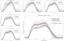
Let us clarify what a spectrally degrading spectral response function is. The figure below shows the absolute spectral response function retrieved for the Meteosat-7 VIS channel. The yellow, purple and green curves mark the retrieval at the beginning, in the mid and at the end of the 20 years mission i.e. 100, 3600 and 7100 days after launch. (Try not to look at the blue curve, the grey stripes and the red dots – they do not matter here.) We can see clearly that the spectral response function degraded stronger in the blue than in the red part of the spectrum and faster in the first half of the mission than in the second.

The coloured shading of each retrieved spectral response curve in the figure above displays an uncertainty, which represents the standard deviation of the retrieval errors. The figure below illustrates how these retrieval errors are correlated spectrally.

Almost certainly, you will require the relative i.e. the maximum-normalised form of a spectral response function but not the absolute form displayed above. But don’t worry, the FIDUCEO project provides you with all spectral response curves and associated spectral error covariance matrices in relative form.
First example
Your retrieval scheme computes the weighted integral of Earth-reflected spectral radiance, like
L(t) = \int \phi(t,\lambda)\,L(\lambda)\,\mathrm{d}\lambda \quad
where \phi(t,\lambda) denotes the relative spectral response function at time t and L(λ) denotes Earth-reflected spectral radiance. Computationally,the above integral is usually discretized. Let \boldsymbol{\phi}(t)=(\phi(t,\lambda_1 ),\dots,\phi(t,\lambda_n ))^\mathrm{T} denote the discretized relative spectral response function at time tt, which is included with the FIDUCEO spectral response datasets, and let \boldsymbol{L}=(L(\lambda_1 ),\dots,L(\lambda_n ))^\mathrm{T} denote the discretized Earth-reflected spectral radiance. Then
L(t) = h\,\boldsymbol{\phi}(t)\cdot\boldsymbol{L}\quad
where “ h ” denotes the spectral resolution of the discretization and “⋅” denotes the dot product of two vectors. The error variance of L(t) is
V(L(t)) = h^2\,\boldsymbol{L}\cdot \left(\boldsymbol{V}(\boldsymbol{\phi}(t))\, \boldsymbol{L}\right) \quad
where \boldsymbol{V}(\boldsymbol{\phi}(t)) designates the discretized spectral error covariance matrix, which is included with the FIDUCEO spectral response datasets.
Second Example
Your retrieval scheme computes the ratio of Earth-reflected radiance to solar irradiance, like
r(t) = \frac{\int \phi(t,\lambda)\,L(\lambda)\,\mathrm{d}\lambda}{ \int \phi(t,\lambda)\,E(\lambda)\,\mathrm{d}\lambda} \quad.
Numerically, the above ratio is usually discretized. Let \boldsymbol{E}=(E(\lambda_1 ),\dots,E(\lambda_n))^\mathrm{T} denote the discretized solar irradiance, then
r(t) = \frac{\boldsymbol{\phi}(t)\cdot\boldsymbol{L}}{ \boldsymbol{\phi}(t)\cdot\boldsymbol{E}} \quad.
The error variance of r(t) is
V(r(t)) = \boldsymbol{g}(t)\cdot \left(\boldsymbol{V}(\boldsymbol{\phi}(t))\, \boldsymbol{g}(t)\right)
with
\boldsymbol{g}(t) = \frac{(\boldsymbol{\phi}(t)\cdot\boldsymbol{E})\,\boldsymbol{L} – (\boldsymbol{\phi}(t)\cdot\boldsymbol{L})\,\boldsymbol{E}}{ (\boldsymbol{\phi}(t)\cdot\boldsymbol{E})^2} \quad.
Now, if your retrieval scheme uses precomputed lookup tables to calculate quantities like integrated Earth-reflected radiance for a certain time-independent spectral response function, you have two options to adapt it to the use of time-dependent spectral response functions. Firstly, you may precompute lookup tables that yield Earth-reflected spectral radiance, which is independent of any sensor spectral response function because the physics on Earth does not depend on the satellite. Then, in your retrieval scheme, you compute integrated Earth-reflected radiance and associated error variance as in the first example. Secondly, you may precompute lookup tables for quantities like integrated Earth-reflected radiance and its ratio to integrated solar irradiance (and the associated error variance) as made explicit in the two examples above for multiple instants in time.
The FIDUCEO project provides MVIRI VIS in-flight spectral response functions at nanometre spectral resolution every 45 days. Hence, even if your retrieval scheme does fit into one of the two “easy” pieces above, adapting it to the use of time-dependent spectral response functions will need considerably more (though not unmanageably more) computer memory. Depending on your retrieval, adaptation may not result in a significant increase of computational time.
And if your retrieval scheme does not fit into the “easy” pieces, think about it and consult us!