How good should a Fundamental Climate Data Record be?
by Rob Roebeling
There is currently an ongoing debate about the exact definition of a Fundamental Climate Data Record. What can the users expect when they obtain a Fundamental Climate Data Record? How should they use it? For what applications can they use it?
In other words: how good should it be?
The current definition of a Fundamental Climate Data Record is: “a long-term data record of calibrated and quality-controlled sensor data designed to allow the generation of homogeneous products that are accurate and stable enough for climate monitoring”. Although the definition seems clear enough, there is still room for interpretation. This is because the wording used is not quantitative. The reader does not know how long ‘long-term’ is, when a data record can be considered homogeneous, or when a data record is accurate and stable enough for climate applications. Thus, there is a risk of misinterpretation.
I’d like to focus on the phrase ‘long-term’. This should be interpreted in relation to the application it is serving. For climate monitoring, or climate analysis, it is important that the climate data record is long enough to capture realistic inter-annual variability. The required length depends on the climate variable that is considered and the systematic and random uncertainty of that climate data record. For a climate variable that behaves smoothly in time and space and shows a distinct temporal trend, for example CO2, the time-series does not need to be very long to detect the climate signal. In case of a very well-calibrated climate data record, a period of 10 years or less would suffice.
The situation gets trickier for climate variables that are highly variable in time and space and don’t show a distinct temporal trend. Cloud amount and precipitation are examples of these. The inter-annual trends of these variables are even more difficult to detect because years with extreme weather changes, such as the El Niño or La Niña years. Even with a perfectly accurate climate data record it will take a long time before we can detect a climate trend in these parameters. One can imagine that the required length of the climate data record will become even longer when one tries to detect climate trends using climate data records with higher systematic and random uncertainties (i.e. that are less accurate).
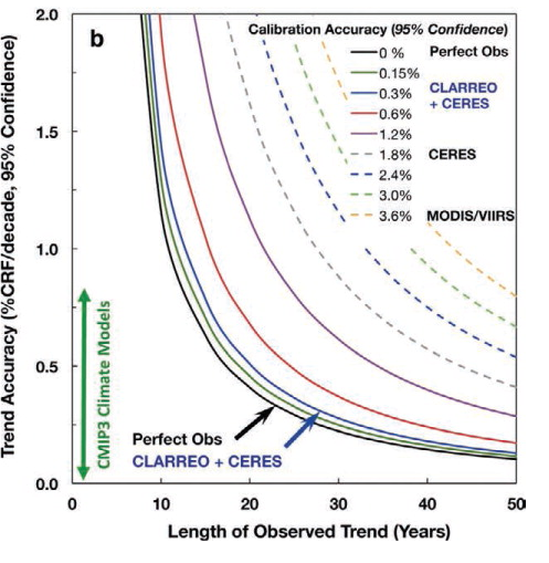
In the paper written by Wielicki, et al. in 2013, a figure is presented that nicely visualises how the length of the time series required to detect a significant climate trend for a particular climate variable increases with decreasing accuracy of the satellite observations. The figure shows the dramatic effect of instrument accuracy on both climate trend accuracy and the time to detect trends (Wielicki, et al., 2013). For example, it would take at least 12 years of perfect observations to detect a trend of 0.8% per decade in cloud radiative forcing. Note, this is the strongest, and, thus, easiest to detect decadal trend as predicted by the models that were part of the third Coupled Model Inter-comparison Project (CMIP3). In the case of observations that have lower calibration accuracies, for example 2.5%, it would take more than 40 years of observations to detect this trend in cloud radiative forcing.
Unfortunately, ‘perfect observations’ do not exist. We can only try to approach the ‘perfect observations’ line by improving the accuracy of our Fundamental Climate Data Records. With the satellite era being ‘only’ about 40 years long this means we need to have Fundamental Climate Data Records that are extremely accurate. The examples shown by Wielicki, et al (2013) show the advantage of improving our calibration accuracy, and that the Fundamental Climate Data Records to be provided by FIDUCEO may really bring into reach the detection of climate trends for more climate variables in the future.
[Fig 1: (See above). The relationship between absolute calibration accuracy and the accuracy of global average decadal climate change trends. Trend accuracy shown for a perfect observing system (black), varying levels of instrument absolute accuracy (solid color lines) for possible CLARREO requirements, and current instruments in orbit (dashed lines). Shown is the relationship between reflected solar spectra and changes in broadband cloud radiative feedback (CRF) and cloud feedback. The green vertical line for reflected solar shows the range of the third Coupled Model Inter-comparison Project (CMIP3) climate model simulations (Soden and Vecchi 2011). Larger values of decadal change in SW CRF indicate larger values of cloud feedback (Soden et al. 2008). (from Wielicki et al. 2013)]
References:
Bruce A. Wielicki, et al., 2013: Achieving Climate Change Absolute Accuracy in Orbit. Bull. Amer. Meteor. Soc., 94, 1519–1539. doi: http://dx.doi.org/10.1175/BAMS-D-12-00149.1
Soden, B. J., I. M. Held, R. Colman, K. M. Shell, J. T. Kiehl, and C. A. Shields, 2008: Quantifying climate feedbacks using radiative kernels. J. Climate, 21, 3504–3520.
Soden, B. J., and G. A. Vecchi, 2011: The vertical distribution of cloud feedback in coupled ocean–atmosphere models. Geophys. Res. Lett., 38, L12704, doi: http://dx.doi.org/10.1029/2011GL047632.