Fast regression considering random errors in all variables
Let’s revisit the example from Sam and Jon’s blog:
Take a straight-line equation Y=A+BX and generate a set of random points (X,Y) that all lie on the straight line with intercept A=0 and slope B=1 . Then add random errors to both X and Y values and fit a straight line to the data. The animated figure below illustrates what happens: ODR takes account of all uncertainties in both X and Y by iteratively varying the straight line and the X value of each data point slightly (indicated by the jiggling blue line and the wobbling yellow triangles) until the vertical distance of the data points from the straight line is “in balance” with the horizontal displacement of the data points from their “measured” position. The eventual straight line has an intercept of A=0 and a slope B=1 with small errors that are consistent with the random errors added to X and Y . (Our animation just illustrates what is varied during the fitting, but does not show how the fitting converges.)
By intention, we discern between jiggling (the straight blue line) and wobbling (the yellow triangles) because the conceptual difference between ODR and simple linear regression is that the former jiggles and wobbles, whereas the latter merely jiggles, which is why it leads to biased solutions.
The animated figure above shows 60 data points, and there is already quite a bit of wobbling apparent . Two parameters are jiggled for the straight blue line, whereas 60 parameters are wobbled for the data. So, there is more wobbling than jiggling.
The harmonisation problem that FIDUCEO is tackling considers some 100 million data points, and ODR must wobble some 100 million yellow triangles, leading to far more wobbling than jiggling. Here ‘jiggling’ specifically refers to the variation of calibration parameters, whereas ‘wobbling’ refers to the variation of satellite state measurements. The solution of the FIDUCEO harmonisation problem by ODR must vary (jiggle) about 60 calibration parameters and (wobble) about 100 million satellite state parameters. In this sense, there is plenty more wobbling than jiggling.
Is there a way to do what ODR does, but without wobbling – just by jiggling, like simple linear regression, but without leading to biased solutions?
We think there is! The general formalism of uncertainty propagation we explained in our November blog makes it possible to transform the uncertainty of the X values into an uncertainty of Y values. The animated figure below illustrates how it works. The straight blue line and the yellow triangles are the same as in the figure above. But here the yellow triangles are not wobbled. Instead, the wobbling of triangles along the X axis is transformed into a stretching and squeezing of shady yellow uncertainty bars along the Y axis. The uncertainty is a function of the slope of the straight blue line: the steeper the slope, the larger the uncertainty. The straight blue line is now jiggled until the vertical distance of the yellow triangles from the straight blue line is “in balance” with the shady yellow uncertainty. (Again, our animation just illustrates what is varied during the fitting, but does not show how the fitting converges.)
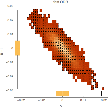
Let’s name our new method “fast ODR”. Then, how do the results of fast ODR compare to those of the ODR method in Sam and Jon’s blog? We have repeated Sam and Jon’s experiment 10,000 times, each time randomly generating thousand (X,Y) points and fitting a straight line by means of fast ODR. The figure below depicts the distribution of the error of the fitted slope B versus the error of the fitted intercept A . We deliberately draw a joint error distribution here, because the errors of the fitted A s and B s are correlated. Like Sam and Jon’s ODR fitting, our fast ODR yields an unbiased solution.
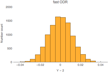
But what happens, if – using the fitted A s and B s – we predict the value of Y at, let’s say, X=2 , a point outside of the fitting domain? Sam and Jon showed that simple linear regression wrongly predicts Y<2 in this case, whereas ODR correctly Y=2 (with a small uncertainty). The figure below illustrates the distribution of the errors of the Y s obtained from fast ODR fitting, which are in very good agreement with the errors of Sam and Jon’s ODR fitting. Both fast and standard ODR give equivalent results!
By means of the same algorithmic differentiation techniques we demonstrated in our November blog, fast ODR can be generalised to apply to the measurement equations of the FIDUCEO harmonisation problem. Our “fast errors-in-variables” implementation solves the (simulated) harmonisation problem for the whole series of AVHRR sensors within less than 400 iterations, in less than 20 minutes on a single workstation computer. Yet, our implementation does not take account of correlated errors.
What is error correlation, how does it arise, and how can it be avoided?
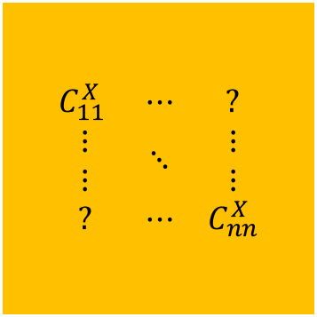
Our first animated figure (that illustrates how ODR works) visualises an error structure that is random: each wobble of an X is independent of all other wobbles of all other X s. If the errors of X were correlated, each wobble would be correlated with some other wobbles, looking like “choreographed dancing” rather than random wobbling. Is considering correlated errors more difficult than considering random errors? Absolutely. The problem is to realise the correct “dance”. Correctly describing the dance of correlated errors in the data for all match-ups requires the computation of some ten quadrillion (10,000,000,000,000,000) numbers. Many of them are simply zero – which unfortunately does neither simplify nor speed-up the problem solving!
So how does error correlation arise? Error correlation between e.g. different image pixels of calibrated radiance arise, if the calibration of different pixels is computed from the same basis data, like the temperature of the internal calibration target or the digital count number recorded for the dark target. Satellite instruments often measure these basic quantities once per row of image pixels, but not per individual pixel. Now, if a match-up data set contains image pixels of the same row, the errors of the calibrated radiance of these pixels are correlated. These type of error correlations in a data set can be avoided only, if the data set does not include multiple image pixels of the same row. Whether such a “clearing” of data sets to avoid error correlation is feasible depends on the number of match-up pixels needed to achieve the accuracy and stability requirements on a calibration.
Another sort of error correlation arises, if images of calibrated radiance are computed from basis data, which are averaged over many image rows: the temperature of the internal calibration target or the digital count number from the dark target are often averaged over several image rows to reduce the uncertainty of the computed calibrated radiance. In fact, the calibrated radiance images look smoother with averaging of these basis data than without, suggesting less uncertainty. But is the uncertainty truly less? No – it isn’t! Instead, the uncertainty of an individual datum is smoothly distributed across many data. In consequence, these calibrated radiance images, though appearing smooth, are not more certain than those without averaging, but with an error structure like choreographed “dancing and singing” that is much more problematic to take account of. Avoiding this entertainment is, however, easy: don’t average your basis data, and the error structure of your derived data will be an easy-to-operate uncorrelated wobbling.
Whether wobbling (graciously) or dancing, FIDUCEO has mastered the former (by means of two independent errors-in-variables implementations) and is approaching the latter. Ultimately, only one question matters: Is the error structure of our climate data records adequately characterised, or not?