An orbit is the gravitationally curved path of an object about a point in space (Wikipedia). Satellites orbiting around Earth are among our most valuable tools for meteorology and earth science in general. Possibilities for Earth orbits are endless, but most of our existing earth observation satellites have one of only two special orbit types: geosynchronous or sun-synchronous. The former, more commonly called geostationary, has the satellite in the equatorial plane, with an altitude chosen such that the satellite moves with the same speed as Earth rotates, so that seen from Earth the satellite seems to hover above a fixed point on the equator.
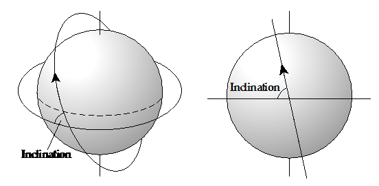
We will not consider the geosynchronous type further here, but instead focus on the other, the sun-synchronous orbit type. This is the type used by the NOAA and MetOp satellites that carry the AMSU-B and MHS instruments, used by FIDUCEO. Sun-synchronous means that these orbits are such, that the satellite passes a given point on Earth always at the same local time. These satellites have a low altitude (they are close to Earth) and a high inclination (angle between the orbit plane and the equatorial plane). Figure 1 shows an example. We characterize these orbits by their altitude, their inclination, and by the local time at which they cross the equator in the northward direction.
Figure 1: A satellite in a high inclination orbit around Earth. (Figure courtesy Oliver Lemke)
Sun-synchronous orbits
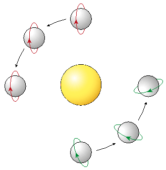
From simple physics (conservation of angular momentum), one might expect the satellite orbit plane to be fixed. For such an orbit the equator crossing local time would change by approximately four minutes every day (by 24 hours in one year), because Earth itself orbits around the sun, as illustrated by the red orbit in Figure 2.
Figure 2: Fix orbit (red) and sun-synchronous orbit (green). (Figure courtesy Oliver Lemke)
If Earth was a perfect sphere, we simply would have to live with this. But Earth is actually a bit oblate (wider than tall) and this causes orbits around it to precess, which means to slowly turn. We can exploit this effect to make the orbit precess exactly once over the course of a year, as illustrated by the green orbit in Figure 2. Such an orbit is sun-synchronous, it keeps its angle towards the sun, and hence its local time of equator crossing. The precession speed depends on orbit altitude and inclination, so for a given altitude there is a ‘magic’ inclination that makes it sun-synchronous.
Orbit drift
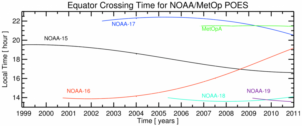
To maintain a sun-synchronous orbit over a long time-period, a satellite has to actively correct its position now and then. Without such active control, the satellite will be nearly sun-synchronous, but its local time of equator crossing will slowly drift over the years of its operation. This can be seen in Figure 3, which shows the long-term evolution of equator crossing local times for some of the microwave satellite sensors that we work on in FIDUCEO. NOAA satellites are not actively controlled, so they drift. MetOp satellites, on the other hand, are actively controlled and do not drift.
Figure 3: The drift in the local time when the satellite crosses the equator in the northward direction. This is Figure 4 of John, V. O., G. Holl, S. A. Buehler, B. Candy, R. W. Saunders, and D. E. Parker (2012), Understanding inter-satellite biases of microwave humidity sounders using global simultaneous nadir overpasses, J. Geophys. Res., 117(D2), D02305, doi:10.1029/2011JD016349.
Diurnal cycle aliasing
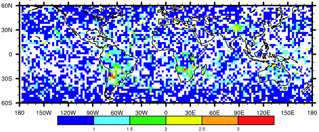
Many atmospheric parameters have a diurnal cycle, that is, they exhibit a typical variation pattern with a one day period. A good example is land surface temperature, which increases during the day, due to heating by solar (shortwave) radiation. During the night, land surface temperature decreases, because of cooling by thermally emitted (longwave) radiation. Upper tropospheric humidity, the subject of one of the FIDUCEO climate data records (CDRs), also has a diurnal cycle in some areas, as demonstrated by Figure 4. We think that this is mainly due to the diurnal cycle of convection over land, which is related to the diurnal cycle of surface temperature.
Figure 4: Amplitude (in Kelvin) of the 24 h period component of the diurnal cycle in the brightness temperature of the innermost microwave humidity channel, used for deriving upper tropospheric humidity (UTH). Data from several different satellites were combined to derive this figure. This is from Figure 4 of Kottayil, A., V. O. John, and S. A. Buehler (2013), Correcting diurnal cycle aliasing in satellite microwave humidity sounder measurements, J. Geophys. Res., 118(1), 101–113, doi:10.1029/2012JD018545.
One of the main problems of constructing satellite CDRs results from the combination of such diurnal cycles and the satellite orbit drifts. Because of the slow drift in local time, different phases of the diurnal cycle are sampled over time, as illustrated in Figure 5. As the figure shows, this will lead to spurious trends if the effect is not accounted for. The phenomenon is called diurnal cycle aliasing.
Figure 5: A schematic drawing illustrating the effect of diurnal cycle aliasing on a long-term trend. The local time of sampling changes slowly over time, and because of this there appears to be a trend in the data (green line), although there really is no trend. (Figure courtesy Oliver Lemke)
In previous efforts to construct satellite CDRs, scientists have attempted to simultaneously correct for instrument calibration offsets and diurnal cycle aliasing. But the two effects are fundamentally different, and naïve corrections thus may introduce new artifacts. The overall lack of traceability in these efforts has lead to disputes that were long and hard to resolve, for example in the case of microwave tropospheric temperature measurements.
In the FIDUCEO community, we think that the only way to resolve these disputes is to attempt to disentangle the two issues, instrument offsets and differences in sampling, for which local time is an example. We are first constructing a fundamental climate data record (FCDR) where the data is harmonized (instrument well calibrated to the best of our ability). In a second step, the FCDRs are used to construct CDRs where the data are homogenized, that is, known sampling differences are corrected for and the residual error is characterized. The benefit of this approach is that it will lead to robust and traceable error estimates, which so far have been lacking.